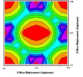
Figure 2: BCC [1 1 0] Contour Plot
Justin Barker
ESM 4984
As a material fractures, plastic deformation typically occurs within the material. The degree to which this plastic deformation occurs is termed ductility. Materials that exhibit little plastic deformation (less then 5% strain) upon fracture are termed brittle, while those that exhibit greater plastic deformation are termed ductile. By examining the deformations that occur in iron at the atomistic level we gain a better appreciation for their failure characteristics.
When plastic deformation is created by dislocation motion it is termed slip. This slip occurs along the slip plane as a result of an applied shear force. As the dislocation moves it creates a series of stacking faults in the material. The stacking faults created can lead to an increase of the surface energy or of the stacking fault energy. As this energy increases the material begins to weaken.
In this exercise my partner (Matt McMurtry) and I
examined the BCC [1 1 0] plane of iron. We ran computer models that
simulated shearing stresses in the x and z axes. The x displacements
ranged from 0 to 0.9*Sqrt(2)*a, and the z displacements ranged from 0 to
0.9*a (where a= the lattice parameter of 2.87 Angstroms). One hundred
combinations of these values were run and the results are tabulted in Figure
1. All values are listed in units of J/m^2.
| X,Z | 0 | 0.406 | 0.812 | 1.218 | 1.624 | 2.029 | 2.435 | 2.841 | 3.247 | 3.653 | 4.059 |
| 0 | 5.86E-14 | 2.77E-03 | 1.16E-02 | 4.31E-02 | 5.03E-02 | 8.26E-02 | 5.03E-02 | 4.31E-02 | 1.16E-02 | 2.77E-03 | 5.86E-14 |
| 0.287 | 3.52E-03 | 6.27E-03 | 1.50E-02 | 3.05E-02 | 6.29E-02 | 6.02E-02 | 6.29E-02 | 3.05E-02 | 1.50E-02 | 6.27E-03 | 3.52E-03 |
| 0.574 | 1.44E-02 | 1.71E-02 | 2.58E-02 | 4.44E-02 | 3.59E-02 | 3.32E-02 | 3.59E-02 | 4.44E-02 | 2.58E-02 | 1.71E-02 | 1.44E-02 |
| 0.861 | 3.32E-02 | 3.59E-02 | 4.44E-02 | 2.58E-02 | 1.71E-02 | 1.44E-02 | 1.71E-02 | 2.58E-02 | 4.44E-02 | 3.59E-02 | 3.32E-02 |
| 1.148 | 6.02E-02 | 6.29E-02 | 3.05E-02 | 1.50E-02 | 6.27E-03 | 3.52E-03 | 6.27E-03 | 1.50E-02 | 3.05E-02 | 6.29E-02 | 6.02E-02 |
| 1.435 | 8.26E-02 | 5.03E-02 | 2.71E-02 | 1.30E-03 | 2.77E-03 | 5.86E-14 | 2.77E-03 | 1.30E-03 | 2.71E-02 | 5.03E-02 | 8.26E-02 |
| 1.722 | 6.02E-02 | 6.29E-02 | 3.05E-02 | 1.50E-02 | 6.27E-03 | 3.52E-03 | 6.27E-03 | 1.50E-02 | 3.05E-02 | 6.29E-02 | 6.02E-02 |
| 2.009 | 3.32E-02 | 3.59E-02 | 4.44E-02 | 2.58E-02 | 1.71E-02 | 1.44E-02 | 1.71E-02 | 2.58E-02 | 4.44E-02 | 3.59E-02 | 3.32E-02 |
| 2.296 | 1.44E-02 | 1.71E-02 | 2.58E-02 | 4.44E-02 | 3.59E-02 | 3.32E-02 | 3.59E-02 | 4.44E-02 | 2.58E-02 | 1.71E-02 | 1.44E-02 |
| 2.583 | 3.52E-03 | 6.27E-03 | 1.50E-02 | 3.05E-02 | 6.29E-02 | 6.02E-02 | 6.29E-02 | 3.05E-02 | 1.50E-02 | 6.20E-03 | 3.52E-03 |
| 2.87 | 5.86E-14 | 2.77E-03 | 1.16E-02 | 4.31E-02 | 5.03E-02 | 8.26E-02 | 5.03E-02 | 4.31E-02 | 1.16E-02 | 2.77E-03 | 5.86E-14 |
The energies calculated with the computer software can be plotted in a contour plot developed using Mathematica. Figure 2 shows this plot. The red values are the areas containing the lowest energy, and the purple area indicate the areas of greatest energy.
Figure 2: BCC [1 1 0] Contour Plot
This data can also be represented in a 3D plot as shown in Figure 3.
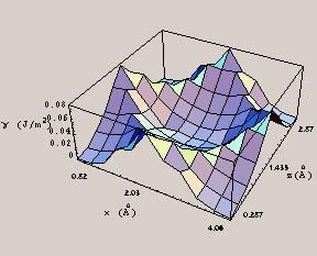
Figure 3: BCC [1 1 0] 3D Plot
The maximum surface energy developed in this mdel was about 0.08 J/m^2. Published values for these energies are approximately 0.06 J/m^2. This is a fairly close correlation.
References
Callister, William D., Jr. Materials Science and Engineering, an Introduction.
4th ed. New
York:
John Wiley & Sons, 1997.
Hull, Derek. Introduction to Dislocations 2nd ed. Oxford: Pergamon
Press, 1975.