Deformation Field in an Axially Loaded Bar

For simplicity we consider a uniform prismatic bar made of a homogeneous and isotropic linear elastic material with its mantle free of surface tractions. One end of the bar is loaded by uniformly distributed surface traction, $\sigma$, acting along the axis of the bar, the centroid of the other end is rigidly clamped to prevent rigid motion of the bar, and the clamped end is loaded to keep the bar in equilibrium. A sketch of the problem studied is shown in Fig. 11.1

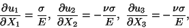
The stress field

$$\sigma_{11} = \sigma,\ \sigma_{22} = \sigma_{33} = \sigma_{12} = \sigma_{23} = \sigma_{31} = 0 \tag{11.1}$$ (11.1)

identically satisfies the equations of equilibrium when gravitational forces are neglected. Also, the traction boundary conditions on the mantle and the loaded end are satisfied. From Hooke's law (6.3) with C given by (6.4), we obtain

$$e_{11} = \frac{\sigma}{E},\ e_{22} = - \frac{\nu\sigma}{E},\ ... ...frac{\nu \sigma}{E},\ e_{12} = e_{23} = e_{31} = 0. \tag{11.2}$$ (11.2)

Therefore

$$\frac{\partial u_1}{\partial X_1} = \frac{\sigma}{E},\ \frac{... ...\partial u_3}{\partial X_3} = - \frac{\nu\sigma}{E},\tag{11.3}$$ (11.3)

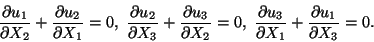$$\frac{\partial u_1}{\partial X_2} + \frac{\partial u_2}{\part... ...artial X_1} + \frac{\partial u_1}{\partial X_3} = 0.\tag{11.4}$$ (11.4)

An integration of equations (11.3) gives
$$\begin{gather}\begin{split} &u_1 = \frac{\sigma}{E} X_1 + f_1(X_2,X_3),\\ &u_2 ... ...3 = - \frac{\nu\sigma}{E}X_3 + f_3 (X_1,X_2). \end{split}\tag{11.5} \end{gather}$$
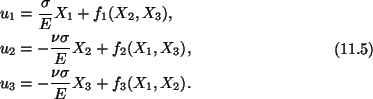
Substitution from (10.5) into (10.4) yields

$$\frac{\partial f_1}{\partial X_2} + \frac{\partial f _2}{\par... ...rtial X_1} + \frac{\partial f_1}{\partial X_3} = 0. \tag{11.6}$$ (11.6)

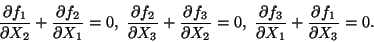
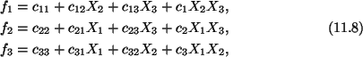
Recalling that f₁ is a function of X₂ and X₃, f₂ is a function of X₁ and X₃, and f₃ is a function of X₁,X₂, we conclude from (11.6) that

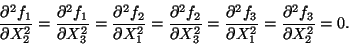$$\frac{\partial^2f_1}{\partial X^2_2} = \frac{\partial^2f_1}{\... ...l X^2_1} = \frac{\partial^2f_3}{\partial X^2_2} = 0.\tag{11.7}$$ (11.7)

Hence
$$\begin{gather}\begin{split} &f_1 = c_{11} + c_{12} X_2 + c_{13} X_3 + c_1X_2X_3,... ... c_{33} + c_{31} X_1 + c_{32}X_2 + c_3X_1X_2, \end{split}\tag{11.8} \end{gather}$$
where $c_{11},c_{12},\ldots c_{32}$, $c_1,\ c_2$ and c₃ are constants. We now substitute from (11.8) into (11.6) to obtain
$$\begin{gather}\begin{split} &(c_{12} + c_{21}) + (c_1 + c_2)X_3 = 0,\\ &(c_{23}... ...,\\ &(c_{31} + c_{13}) + (c_3 + c_1)X_2 = 0. \end{split}\tag{11.9} \end{gather}$$
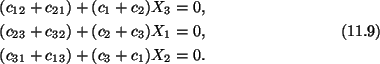
Since these equations must hold for all points in the interior of the bar, therefore
$$\begin{gather}\begin{split} &c_{12} = - c_{21},\ c_{23} = - c_{32},\ c_{31} = - ... ...},\\ &c_1 + c_2 = c_2 + c_3 = c_3 + c_1 = 0.\end{split}\tag{11.10} \end{gather}$$
The second set of equations (11.10) gives

c₁ = c₂ = c₃ = 0. (11.11)

Substitution from (11.8), (11.10) and (11.11) into (11.5) gives the following expressions for the displacement field in the bar.
$$\begin{gather}\begin{split} &u_1 = \frac{\sigma}{E}X_1 + c_{12}X_2 + c_{13}X_3 +... ...gma}{E}X_3 - c_{13}X_1 - c_{23}X_2 + c_{33}. \end{split}\tag{11.12} \end{gather}$$
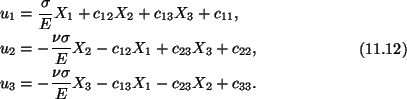
Since u₁ = u₂ = u₃ = 0 at the centroid X₁ = X₂ = X₃ = 0of the bar, therefore, we conclude from (11.12) that

c₁₁ = c₂₂ = c₃₃ = 0. (11.13)

In order to eliminate rigid rotations of the bar,

$$\left(\frac{\partial u_1}{\partial X_2} - \frac{\partial u_2}... ...u_1}{\partial X_3}\right)\bigg\vert _{(0,0,0)} = 0.\tag{11.14}$$ (11.14)

That is, a small region around the centroid of the cross-section at X₃ = 0 is rigidly clamped. Equations (11.12) and (11.14) give

c₁₂ = c₁₃ = c₂₃ = 0. (11.15)

Thus, the displacement field in the bar is given by

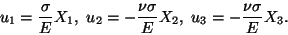$$u_1 = \frac{\sigma}{E}X_1,\ u_2 = - \frac{\nu\sigma}{E}X_2,\ u_3 = - \frac{\nu\sigma}{E}X_3. \tag{11.16}$$ (11.16)

If the diameter of the cross-section of the bar is much smaller than the length of the bar, then the maximum values of u₂ and u₃ will be considerably smaller than the maximum value of u₁. In such cases, we neglect changes in the cross-section of the bar and focus on finding u₁only.

Consider a bar for which the Young's modulus is a function of X₁, and a typical dimension in the cross-section is much smaller than the length of the bar. We will neglect lateral deformations of the cross-section and find u₁ = u only as a function of X₁ = X. Equations for finding the function uare
$$\begin{gather}\begin{split} &\frac{d\sigma_{11}}{dX} = 0,\ \sigma_{11} = E\frac{... ...= 0,\ \sigma_{11} = \sigma\ {\rm at}\ X = L. \end{split}\tag{11.17} \end{gather}$$
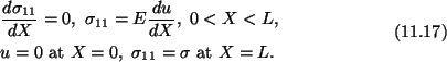
Substitutiion for $\sigma_{11}$ in terms of u gives
$$\begin{gather}\begin{split} &\frac{d}{dX}\left(E\frac{du}{dX}\right) = 0,\ 0 < X... ...(E\frac{du}{dX}\right)\bigg\vert _{X=L} = L. \end{split}\tag{11.18} \end{gather}$$
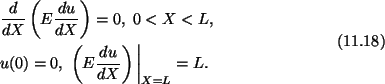
If E as a function of X is known, then we can integrate the second-order ordinary differential equation (11.18)₁ and solve for u. However, when the functional relationship between E and X is complicated, one may not be able to analytically integrate (11.18)₁. We now discuss the finite element method of solving the problem defined by (11.18).

Boundary condition (11.18)₂ is called essential, and (11.18)₃ natural. Instead of directly solving eqn. (11.18) we will first derive the potential energy of the system and find a solution by minimizing the potential energy. As shown in Section 9, the potential energy is minimum in the equilibrium configuration. This approach is being followed to stay consistent with the earlier lectures in this course.

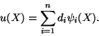
Strain energy of the bar is given by
$$\begin{align}W =\ & A\int^L_0 \frac{1}{2}\sigma_{11}e_{11} dX = \frac{A}{2} \int... ...=\ & \frac{A}{2}\int^L_0 E\left(\frac{du}{dX}\right)^2 dX\tag{11.19} \end{align}$$
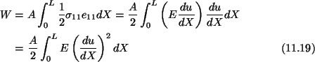
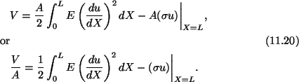
where A is the cross-section of the bar. Since the end X = 0is fixed, therefore, for the potential energy, V, of the system we have
$$\begin{gather}\begin{split} &V = \frac{A}{2}\int^L_0 E\left(\frac{du}{dX}\right)... ...X}\right)^2 dX - (\sigma u)\bigg\vert _{X=L}.\end{split}\tag{11.20} \end{gather}$$
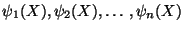
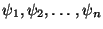
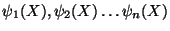
In the finite element work, we express u as a linear combination of the finite element basis functions $\psi_1(X), \psi_2(X),\ldots ,\psi_n(X)$. The given domain is divided into disjoint (nonoverlapping) subdomains, called finite elements so that their union (sum) equals the entire domain. Thus every part of the region is counted only once. Special points generally on the common boundary of adjoining elements are selected and called nodes. The collection of elements and nodes is called a finite element mesh. For the potential energy with first-order derivatives in the integrand, the basis functions $\psi_1,\psi_2,\ldots , \psi_n$ must be once differentiable everywhere on [0,L] except possibly at a finite number of points. Thus these functions must be continuous on [0,L]. Functions $\psi_1,\psi_2,\ldots , \psi_n$ are chosen to satisfy the following conditions: (1) $\psi_i(X)$ equals 1 at node i and vanishes at all other nodes, (2) $\psi_i(X)$ is a simple polynomial defined piecewise over the entire domain, and (3) a constant can be expressed as a linear combination of $\psi_1,\psi_2,\ldots , \psi_n$. Thus for the finite element mesh

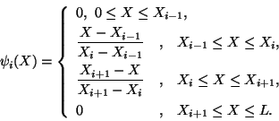$$\psi_i(X) = \left\{\begin{array}{lll} \multicolumn{3}{l}{0, \... ...5in} 0 & , & X_{i+1}\le X \le L.\end{array}\right. \tag{11.21}$$ (11.21)

The basis function $\psi_i(X)$ is non-zero only on the two elements that share node i. The restriction of a basis function to an element is called a shape function, and a basis function $\psi_i$ is obtained by patching together the shape functions defined on elements meeting at node i. Corresponding to basis functions (11.21) there are only two basis functions which are non-zero on an element. For example, on element $\Omega_e$ with nodes e and e + 1, only $\psi_e$ and $\psi_{e+1}$ will be non-zero; $\psi_e$ equals 1 on the left node e and zero on the right node (e + 1) and $\psi_{e+1}$ equals zero on the left node e and 1 on the right node (e + 1). Hence there are two shape functions associated with the element e; one with each node on the element. The shape function for node e equals 1 at node e and zero at node e + 1, and the shape function for node e+1 takes on values 0 and 1 respectively at nodes e and e+1.

Temporarily, we ignore the boundary condition u(0) = 0 and approximate uby

$$u(X) = \sum^n_{i=1} d_i\psi_i(X). \tag{11.22}$$ (11.22)

Recalling that

$$\psi_i(X_j) = \left\{\begin{array}{lll} 1, & {\rm if} & i = j,\\ 0, & {\rm if} & i\ne j,\end{array}\right. \tag{11.23}$$ (11.23)

we get

$$u(X_j) = d_j \equiv u_j\tag{11.24}$$ (11.24)

That is, d_i in (11.23) equals the value of the unknown function at node i. Substitution from (11.22) and (11.24) into (11.20) yields

$$\frac{V}{A} = \frac{1}{2}\sum^{n-1}_{i=1}\int^{X_{i+1}}_{X_i}... ...1}_{k=1}u_k\psi_k(X)\right)\right]\bigg\vert _{X=L}\tag{11.25}$$ (11.25)

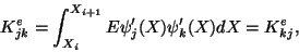
where $\psi^\prime_j (X) = d\psi_j/dX$. For $\psi_i$ given by (11.21), $d\psi_i/dX$ is exhibited in Fig. 11.3. The derivative $\psi^\prime_i(X)$ is undefined only at three points, $X=X_{i-1},\ X_i$ and X_i+1.

Therefore, the integral on the right-hand side of (11.25) can be evaluated. After the other expression on the right-hand side of (11.25) has also been evaluated, V becomes a function of n variables, viz., $u_1,u_2,\ldots , u_n$. The stationary points of V are given by

$$\frac{\partial V}{\partial u_k} = 0,\ k = 1,2,\ldots , n, \tag{11.26}$$ (11.26)

or

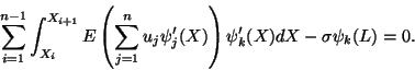$$\sum^{n-1}_{i=1}\int^{X_{i+1}}_{X_i}E\left(\sum^n_{j=1}u_j\ps... ...) \right) \psi^\prime_k(X)dX - \sigma\psi_k(L) = 0.\tag{11.27}$$ (11.27)

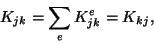
With the notations

$$K^e_{jk} = \int^{X_{i+1}}_{X_i} E\psi^\prime_j (X)\psi^\prime_k (X) dX = K^e_{kj},\tag{11.28}$$ (11.28)

$$K_{jk} = \sum_e K^e_{jk} = K_{kj},\tag{11.29}$$ (11.29)

$$F_k = \sigma\psi_k(L),\tag{11.30}$$ (11.30)

we can write (11.27) as

K_jk u_j = F_k. (11.31)

To see if the stationary points given by (11.26) or equivalently a solution of (11.31) minimizes V, we need to examine the second-order derivatives. Note that

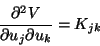$$\frac{\partial^2V}{\partial u_j\partial u_k} = K_{jk}\tag{11.32}$$ (11.32)

and once u(0) = 0 has been used, the matrix Kis positive definite. Thus, indeed the solution of (11.31) minimizes the potential energy V and corresponds to an equilibrium configuration of the body.

The matrix K^e is called the element stiffness matrix, and K the global stiffness matrix. The vector Fis the load vector. For the present problem, Fhas a contribution only from the applied load at the end x = L. This is evidenced by $\psi_k(L)$ equalling 1 only when k = n, and zero otherwise.

We now impose the boundary condition u₁ = 0 or u(0) = 0. One way to accomplish this is to delete the first row and first column of the matrix K, and the first row of F, and then solve (11.31) for the remaining unknowns $u_2,u_3,\ldots , u_n$. The other technique is to add a big number B to K₁₁ and Bu(0) to the first column of F, and then solve (11.31) for $u_1,u_2,\ldots , u_n$. In this case the boundary condition u(0) = 0 is approximately satisfied. Knowing $u_1,u_2,\ldots , u_n$, the displacement u at any point in the bar is found from

$$u=u_1\psi_1(X) + u_2\psi_2(X) + \ldots + u_n\psi_n(X) \tag{11.33}$$ (11.33)

where $\psi_1(X),\psi_2(X)\ldots \psi_n(X)$ are the known finite element basis functions. One can compute the axial strain $e_{11} = \displaystyle\frac{\partial u}{\partial X}$ from (11.33) and then the axial stress $\sigma = E\displaystyle\frac{\partial u} {\partial X}$ at any point in the bar. Since the basis functions $\psi_1(X), \psi_2(X),\ldots ,\psi_n(X)$ are not differentiable at the node points, therefore strains and stresses can not be computed there. Stresses are computed at points interior to an element, and are extrapolated to nodes if needed.

The basis functions shown in Fig. 11.2 are polynomials of order one in x. These are lowest order polynomials that can be used to solve the present problem. However, higher order polynomials defined piecewise over the domain that are continuous across neighboring elements will work too, and will usually give a better representation of the axial stress than that obtained with polynomials (11.21). Another way to improve the accuracy of the solution is to use a finer mesh, i.e., reduce the size of the elements.