


Next: About this document ...
Up: No Title
Previous: Deformation Field in an
Consider deformations of a straight prismatic bar made of a homogeneous linear
elastic isotropic material due to a pair of couples of magnitude M applied
to the ends of the beam. Because of symmetry, the problem is equivalent to
that a cantilever beam loaded by a couple at one end. The couple M is caused
by distributed surface tractions acting on the end faces. The resultant force
of these tractions is zero, and their moment equals M about the X2-axis
(see Fig. 12.1). The line passing through the centroids of the
cross-sections of the beam is called the central line. Assume that plane
sections of the beam normal to the central line before deformation remain
plane and normal to the deformed central line. For the co-ordinate axes shown
in Fig. 12.1 with X3-axis coincident with the central line, assume that
the stresses in the beam are given by
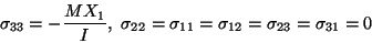 |
(12.1) |
where I is the moment of inertia of the cross-section about the X2-axis.
The assumed stress field satisfies the equilibrium equations (3.11). To see
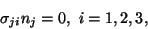
if the boundary conditions are also satisfied, we note that on the lateral
surface of the bar,
n = (n1,n2,0),
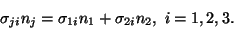 |
(12.2) |
For the stress field given by (12.1),
 |
(12.3) |
on the lateral surface of the bar. On the end face X3 = L,
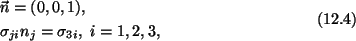
which is non-zero only for i = 3. For i= 3,
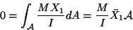
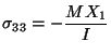 and the boundary condition of zero resultant
axial force
requires that
and the boundary condition of zero resultant
axial force
requires that
 |
(12.5) |
where  is the area of cross-section of the bar and
 is the X1 coordinate of the centroid of the cross-section.
Since X3-axis coincides with the central line,
is the X1 coordinate of the centroid of the cross-section.
Since X3-axis coincides with the central line,
 . The moment
about the X2-axis of surface tractions on the end-face X3=L should equal
the applied bending moment M. Thus
. The moment
about the X2-axis of surface tractions on the end-face X3=L should equal
the applied bending moment M. Thus
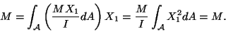 |
(12.5) |
Since point-wise traction type boundary conditions are not
satisfied on the end face X3 = L, the assumed stress state (12.1) and hence
the displacements computed below from it are not valid in the immediate
vicinity of this surface. According to St. Venant, however, the solution
(12.1) is good at points far away from the end face X3 = L.
We now compute the displacement field, find the deformed shape of the bar, and
satisfy displacement type boundary conditions at X3 = 0. Using Hooke's law
(6.3) with
C given by (6.4), we obtain
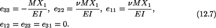
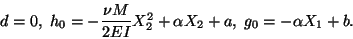
Substitution from (12.7) into the strain-displacement relations (5.13) gives
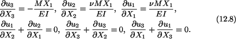
An integration of (12.8)1 results in
 |
(12.9) |
Substituting from (12.9) into (12.8)5 and (12.8)6 we obtain
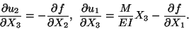 |
(12.10) |
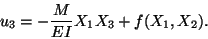
Hence
 |
(12.11) |
where g and h are unknown functions of X1 and X2. We
now substitute from (12.11) into (12.8)2 and (12.8)3 to obtain
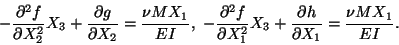 |
(12.12) |
Since these equations hold for all values of X3, therefore
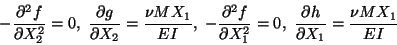 |
(12.13) |
An integration of these equations gives
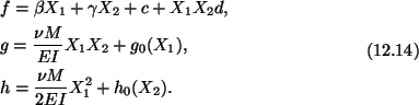
Substituting from (12.13) into (12.10) and the result into
(12.7)4 we arrive at
 |
(12.15) |
This equation holds at every point in the bar if only if
 |
(12.16) |
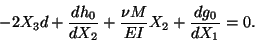
Thus
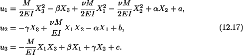
Constants
 and
and  represent the
rigid motion of the bar. In order to determine these, we fix the beam at the
origin, fix an element of the X3-axis, and an element of the X1X3-plane
at the origin. Thus
represent the
rigid motion of the bar. In order to determine these, we fix the beam at the
origin, fix an element of the X3-axis, and an element of the X1X3-plane
at the origin. Thus
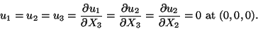 |
(12.18) |
Conditions (12.17) require that
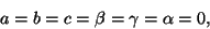 |
(12.19) |
and the displacement field in the beam is given by
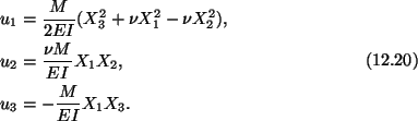
Points on the central line
(X1 = X2 = 0) of the beam are
deformed into the curve
 |
(12.21) |
or into the parabola
 |
(12.22) |
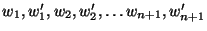
We now analyze the problem by the finite element method. The goal is to find
the deformed shape of the central line. We denote the vertical displacement
of a point by w instead of u1. The first step is to find the potential
energy of the system.
Equation (8.9) gives the strain energy stored in the body. For the present
problem
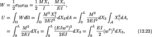
where we have assumed that the cross-section of the beam is
uniform, and
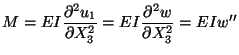 which follows from
(12.19)1. The potential energy of the beam loaded by a couple or moment at
the end X3 = L is given by
which follows from
(12.19)1. The potential energy of the beam loaded by a couple or moment at
the end X3 = L is given by
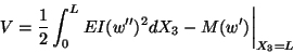 |
(12.24) |
where
 .
.
For the potential energy given by (12.24) to have a finite value, the
second-order derivatives of w must be square integrable. Thus  must be continuous. Recall that the first-order derivatives of the finite
element basis functions used in Section 11 are discontinuous at the node
points. It implies that a different set of finite element basis functions is
needed.
must be continuous. Recall that the first-order derivatives of the finite
element basis functions used in Section 11 are discontinuous at the node
points. It implies that a different set of finite element basis functions is
needed.
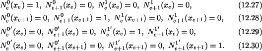
In order to simplify the notation, we set
x3 = X3 = x, and
 .
.
Divide the domain [0,L] into n finite elements with nodes at the
end-points of each element. Thus the coordinates of (n + 1) nodes can be
denoted by
 .
We use
two sets of basis functions - one to make the deflections wcontinuous and the
other to make first-order derivatives of w or the slope
.
We use
two sets of basis functions - one to make the deflections wcontinuous and the
other to make first-order derivatives of w or the slope
 continuous. Recalling that the basis function corresponding to a node i can
be be obtained by patching together the shape functions defined on adjoining
elements meeting at node i, we generate the shape functions below.
continuous. Recalling that the basis function corresponding to a node i can
be be obtained by patching together the shape functions defined on adjoining
elements meeting at node i, we generate the shape functions below.
On the element  with left node xe and right node xe+1, we
write
with left node xe and right node xe+1, we
write
 |
(12.25) |
Here we(x) is the unknown function w defined on the
element , shape functions N0e and N0e+1 ensure the
continuity of we across inter-element boundaries, and shape functions
N1e and N1e+1 are meant to make
continuous
across inter-element boundaries. In order to meet these continuity
requirements, we set
 |
(12.26) |
These are fulfilled if
Since each shape function satisfies four conditions, we assume that
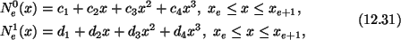
and similar expressions for
N0e+1(x) and
N1e+1(x). We use (12.27)1, (12.28)1,
(12.29)1 and (12.30)1 to obtain four equations for the determination of
 and c4. Expressions for the shape functions so obtained
are given below.
and c4. Expressions for the shape functions so obtained
are given below.
![\begin{gather}\begin{split}&N^0_e(x) = 1 - 3\left(\frac{x - x_e}{h_e}\right)^2 +...
...{h_e}\right)^2 - \frac{x -
x_e}{h_e}\right].
\end{split}\tag{12.32}
\end{gather}](img250.gif)
Note that N0e and N0e+1 are dimensionless but N1eand N1e+1 have dimensions of length. Since N1e and N1e+1multiply slopes and N0e and N0e+1 multiply deflections, every term
in (3.4.1) has the same dimension. Shape functions (12.32) are sketched in
Fig. 12.2, and are called Hermitian.
Writing (12.24) as
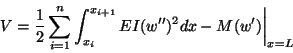 |
(12.33) |
substituting for w from (12.25), and after carrying out the
integration, we will have V as a function of
 . For V to be
stationary,
. For V to be
stationary,
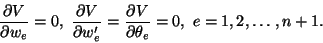 |
(12.3.4) |
Equations (12.34) are equivalent to
where
![\begin{align}&\mathbf{K} = \sum_e\mathbf{K}^e,\nonumber\\
&\mathbf{K}^e = \int^...
...ht] dx.
\nonumber\\
&\mathbf{F} = (0,0,0,0,\ldots , 0,1)M.\nonumber
\end{align}](img255.gif)
For the case of constant EI (e.g. a homogeneous beam of uniform
cross-section), the element stiffness matrix
Ke is given below.
![\begin{displaymath}K^e = \frac{2EI}{h^3_e}\left[\begin{array}{cccc} 6 & -3h_e & ...
...],\ EI = {\rm const},\ h_e = \mbox{element length}
\tag{12.36}
\end{displaymath}](img256.gif) |
(12.36) |
We now apply essential boundary conditions
 in (12.35)
by one of the two methods discussed earlier in Section 11 (e.g. see page 27),
and solve (12.35) for
W. Knowing deflections and slopes at the
node points, we use eqn. (12.25) to find deflections, slopes and curvatures at
any point within an element. The value of the bending stress can then be
computed from
in (12.35)
by one of the two methods discussed earlier in Section 11 (e.g. see page 27),
and solve (12.35) for
W. Knowing deflections and slopes at the
node points, we use eqn. (12.25) to find deflections, slopes and curvatures at
any point within an element. The value of the bending stress can then be
computed from
 .
.
Next: About this document ...
Up: No Title
Previous: Deformation Field in an
Norma Guynn
1998-09-09