Microstructure Lectures

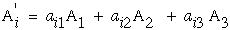
4.1 Introduction to Mechanical Behavior of Anisotropic Materials

In the early part of the 20th century most engineering materials were isotropic. In the later part of the 20th century, 1970s -> 1990s, the aerospace industry created the demand for new, high-strength, high stiffness and light-weight fiber-reinforced composite materials. Because these materials are also highly anisotropic, designers could optimize their designs, i.e. orient the direction of high stiffness and strength in the load direction. Other materials used in "Smart" or "Intelligent" structures, such as piezioelectric polymers are also highly anisotropic. Because the properties of these new materials could be tailored, designers, could for the first time, design the material for the application instead of designing an application around fixed material properties. Anisotropic materials are becoming the material of choice in a variety of engineering applications as we enter the 21st century. Studying the mechanical behavior of these highly anisotropic materials under static and dynamic loads at all scales is relevant when considering current engineering practice.

In the early part of the 20th century anisotropy was more a topic of scientific research then a property used in engineering design. Nye's text on "Physical Properties of Crystal", Ref.[6], gives an excellent introduction to anisotropy in crystals from a material scientist perspective. Lekhnitski's text on "Theory of Elasticity of an Anisotropic Body", Ref.[7], began to address issues of anisotropy in engineering design. In this section we will give a very brief introduction to anisotropy for a continuum (macroscale) and then apply what we learned to anisotropic laminates at the microscale. In section 10.0 we will also show how anisotropy can significantly control dynamic mechanical behavior in a continuum (macroscale).

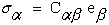
Mechanical behavior of anisotropic materials is characterized in the most general notation as a fourth order stiffness tensor, C_ijkl, which is contracted into a six by six stiffness matrix, C_α,β, relating six components, σ_α, of a symmetric stress tensor to the six components, e_β, of the symmetric strain tensor which are written here as column vectors.

(4)

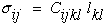
Although this contracted notation shown above is convenient and will be used below to model mechanical behavior of anisotropic laminates at the microscale, a more complete description of elastic anisotropy will require that we return to the more general form where the stiffness matrix that relates strains to stress is written as a fourth order stiffness tensor C_ijkl, where the stresses, σ_ij, and Lagrangian strains, l_ij, must then be written as second order tensors. We will show that this more general tensoral form will allow us to create unique three dimensional geometric representation surfaces for each unique anisotropic elastic symmetry.

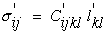
(5)

First we will show how stress can be written in the form of a second order tensor. The proof that stress is a second order tensor because it transforms as a second order tensor is given in Ref.[8].

Figure 7 shows how all possible components of stress acting as forces on a small differential element can be organized into a matrix format which can also be reduced to index notation where i and j are called "free" indices that are assigned values of 1, 2, or 3. All possible combinations of the i and j indices yield the desired three by three matrix.

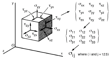
Figure 7. Stress tensor components shown on a differential element

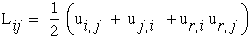
Writing all six components of strain into a similar matrix is not as straight forward as it was for stress where each stress components could be simply seen as a force acting on the surface of a cube. Strain implies displacement which requires much more development, see Ref.[8] Chapter 3, "Analysis of Deformation in a Continuum". Suffice it to say that strain like stress has 9 components which can be identified with the same indices which identifies a displacement direction or shearing in a plane associated with each strain component. From a Lagrangian viewpoint, for large displacement gradients, the nonlinear strain displacement relationships are shown below.

(6)

If we assume only small displacement gradients then the nonlinear terms can be neglected and the upper case "L" is reduced to the lower case "l" which is used to denote the linear lagrangian strain tensor, l_ij.

(7)

With strain and stress defined as second order tensors, it is not difficult to derive the desired linear anisotropic relationship, equation (5), from the first law of thermodynamics. One form of the first law of thermodynamics is shown below.

(8)

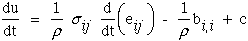
where u is the specific internal energy per unit mass, ρ is the density, e_ij is the Eulerian strain associated with Eulerian displacement gradients, c is the radiative heat transfer per unit time per unit mass, and b_i is the heat transferred through a unit surface per unit time. Note d/dt is the total or comoving derivative. For a complete derivation see Ref.[8], Chapter 4, section 4.5.

If we assume no heat transfer by radiation or conduction and we assume that only small displacement gradients result in lagrangian strains, l_ij, equation (8) reduces to a form where u is now called the strain energy per unit mass since the only mechanism available for storing internal energy in the continuum is through deformation.

(9)

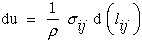
Next let's assume density is constant, or at least a function of strains and that stresses are related to strains by some unknown function (to be determined). Hence strain energy can be a function of stress or strain. For the purpose of discussion here we assume strain energy can be written as some function of strain.

(10)

(11)

Substituting equation (11) into equation (9) yields.

(12)

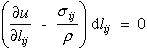
If this relationship is true for any arbitrary nonzero dl_ij, then the relationship in the parenthesis must vanish which yields an equation that shows the relationship between stress, strain and strain energy per unit mass.

(13)

Recall that for equation (10) we assumed some undefined functional form for strain energy as a function of strain. One possible function would be to expand the strain energy into a power series whose coefficients like strain are tensors but constants with indices that sum ("contraction") with the indices of the strain tensors such that each term in the series is a scalar component of the strain energy. The first term α is an arbitrary energy reference state, so we can set it to zero. The second term is a zero strain reference state. The third term is the linear elastic term and the fourth term is the nonlinear, but elastic, term. Higher order terms can be added here as needed to model the desired constitutive stress-strain relationship.

(14)

Substituting this function for strain energy into equation (13) yields the most general form of the anisotropic elastic constitutive law in tensor format.

(15)

NOTE: 1) it is perhaps more evident at this point that the coefficient β;_ij represent the residual stresses when the strains, l_ij, go to zero, and 2) the coefficient δ_ijklmn is the nonlinear elastic term that gives rise to nonlinear elastic stress-strain diagrams not associated with dissipative constitutive models, which we also set to zero. With these simplifications equation (15) reduces to the desired linear-elastic equation.

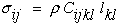(16)

Where C_ijkl are the terms that relate components of strain to the components of stress per unit mass. A similar expression without density can be derived where strain energy per unit volume is introduced into the derivation. Interestingly to remove density is not as straight forward as one might think, see Ref.[8].

(17)

Lets briefly look at an arbitrary geometric transformation of equation (17). For a full development of this type of transformation see Ref.[8]. It can be shown that both stress and strain are second order tensors because they transform as second order tensors and C_ijkl transforms as a fourth order tensor.

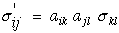(18)

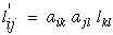(19)

(20)

---

Transformation Law of a vector

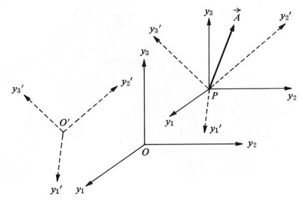
Figure 8. Vector drawn with respect to two different Cartesian axes

Introduce the direction cosines between the two sets of axes:

(a₁₁, a₁₂, a₁₃) = direction cosines of the y^'₁-axis with respect to the (y₁,y₂,y₃)-axes.

(a₂₁, a₂₂, a₂₃) = direction cosines of the y^'₂-axis with respect to the (y₁,y₂,y₃)-axes.

(a₃₁, a₃₂, a₃₃) = direction cosines of the y^'₃-axis with respect to the (y₁,y₂,y₃)-axes.

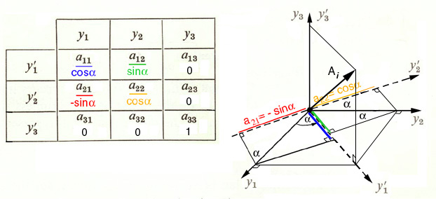
Figure 9. Direction Cosine Matrix With a Simple Rotation About the y₃ axis.

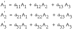
Hence, the relation between the vector A^' and A can be summarized as follows.

(21)

Note that the indices on A^' can be replace as i=1,2,3 hence the three equations in equation (21) reduces to one equation with a "free" index "i".

(22)

Also note that when the number in each term in equation (22) are the same (1 1 in the first term, + 2 2 in the second term, and + 3 3 in the third term) we introduce a new idea of a "summation" notation where any such summation can be notationally simplified and replaced with repeated indices in one term. Hence we can now use this summation index to reduce equation (22).

(23)

---

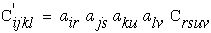
The same direction cosine matrix, a_ij, can also be used in the transformation of stress, strain, and stiffness, in equations (18), (19), and (20) which when substituted into equation (17) reveals that the same equation exists in the arbitrary prime coordinate system, equation (24). The fact that equations (17) and (24) are identical demonstrates that equation (17) is invariant to any ARBITRARY transformation, hence equation (17) is a "tensor equation". The keyword here is arbitrary.

(24)

NOTE ON ARIBITRARINESS: Before we move on to understanding the different types of anisotropies, there is one very important idea that needs to be introduced about equations (17) and (24) which is that tensor equations by definition exhibits mathematical "invariance" to any ARBITRARY transformation. Although the two ideas of invariance and arbitrariness are mathematical ideas, these same ideas of invariance to an arbitrary transformation is also the same fundamental idea, indeed a requirement, of a physical law. Hence invariant arbitrary transformations are essential properties for both physical laws and tensor equations. Are all tensor equations by definition physical laws, is a question that remains unanswered but an interesting topic for discussion.

Equations (17) and (24) are the form of Hooke's Law we need to continue the discussion of anisotropic elasticity by Nye and also to show some interesting "glyphs" (geometric representations) of the fourth order stiffness tensor, C_ijkl .

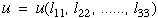
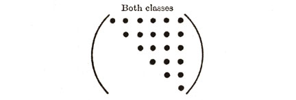
Now that we have introduced elastic anisotropy both as a fourth order tensor and a six-by-six matrix with reduced notation, the reader can now understand the comprehensive treatment of elastic anisotropy given by Nye, Ref.[6], in chapter 8, "Elasticity. Fourth-Rank Tensors", pp. 131-149, where both stiffnesses and compliances are described in terms of matrix and tensor notation. Our objective here is to summarize and highlight the different elastic anisotropies commonly encountered by todays materials engineers. Figure 10 summarizes the various elastic anisotropies in matrix notation.

KEY TO NOTATION
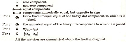TRICLINIC (21)
MONOCLINIC (13)
ORTHORHOMBIC (9)                       CUBIC (3)
(7)          TETRAGONAL          (6)
(7)             TRIGONAL             (6)
HEXAGONAL (5)                          ISOTROPIC (2)

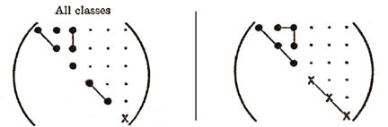Figure 10. Various anisotropies for S_ij and C_ij.

As shown in Figure 10, the different elastic anisotropies are related to the number of independent terms in the elastic property matrix where symbols represent either stiffnesses or compliances. Each of these unique matrices can be related to crystal symmetry classes but here we will discuss just a few of the major classes and symmetry conditions. Triclinic is the most general with 21 independent components. Starting with Triclinic the number of independent terms can be reduced using symmetry planes and invariant rotations. For example if we could imagine ourselves standing inside a crystal and observed that the crystal structure looked identical if we looked either in the +z or -z direction. With this observation we would conclude that symmetry exists about the x-y (1-2) plane and the transformation matrix, a_ij, would be the identity matrix but with the term a₃₃ set equal to -1, see Figure 11. Using this transformation matrix in equation (17) components of the stress tensor are compared in the primed and unprimed coordinates.

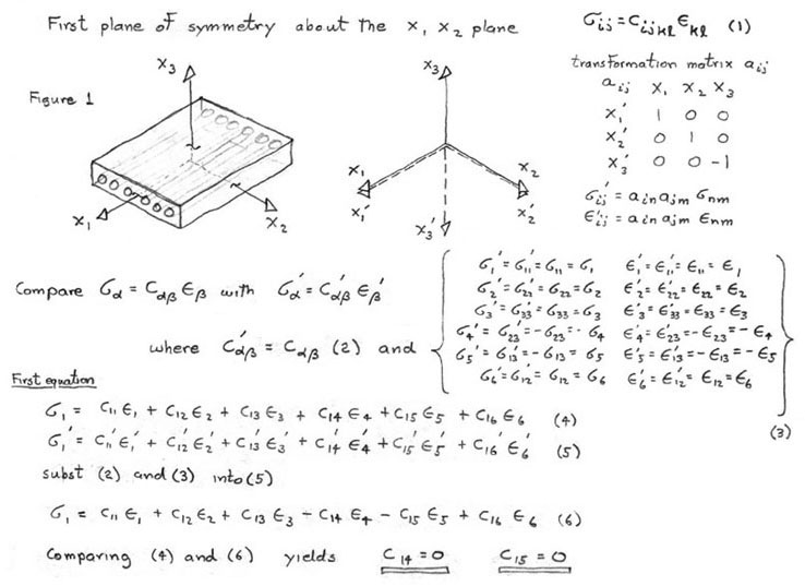
Figure 11. Sample calculation of transformation for symmetry about the x-y (1-2) plane.
NOTE: transformation of stress and strain requires the use of tensor transformations
eqns. (18) and (19) to get the correct sign.

This comparison determines which matrix terms must vanish. For example in Figure 11 comparing σ₁ with σ₁^' requires C₁₄ and C₁₅ vanish. Similar comparisons with the other stress components requires,

(25)

Hence this reduces the Triclinic with 21 independent terms to Monoclinic with 13 independent terms. Figure 10 shows two different types of Monoclinic matrices. If we continue with symmetry in the x-z and y-z plane additional terms must vanish and Monoclinic reduces to Orthotropic with 9 independent terms. Arbitrary rotation about the z axis (3-direction) assuming elastic properties are invariant reduces Orthorhombic to Hexagonal with five independent terms. Of course for isotropic there are only two independent terms or components of the stiffness or compliance fourth order tensor.

Elastic symmetries commonly encountered when working with fiber-reinforced materials commonly used in lightweight aircraft and aerospace structures, are called "orthotropic" which is the same as orthorhombic and "transversely isotropic" which is equivalent to hexagonal.

We continue the development of anisotropic mechanical behavior into two sections. First we focus on engineering elastic properties and represent anisotropy in terms of engineering properties: E, G, and ν, and second we focus on all components of the fourth order stiffness tensor. In both cases we ephasize the use of geometry to study the anisotropy.