Strain Tensors

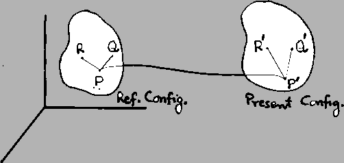
As seen in the previous section, during the motion of a deformable continuum, material lines originating from a material point are rotated and stretched. Whenever the material lines emanating from a material point are stretched and/or the angle between two different material lines passing through a material point changes, the body is said to be strained or deformed. We have seen in the previous section that the deformation gradient is a measure of the stretch and rotation of various material vectors. In this section we will introduce two more measures of deformation which, of course, will be related to the deformation gradient.

Consider two material vectors $\mathbf{P}\mathbf{Q}$ and $\mathbf{P}\mathbf{R}$ originating from the material point $P(X_A)$ in the reference configuration. Let $\mathbf{P}\mathbf{Q}$ be deformed into $\mathbf{P}^\prime \mathbf{Q}^\prime$ and $\mathbf{P}\mathbf{R}$ into $\mathbf{P}^\prime\mathbf{R}^\prime$. Then

$$(P^\prime Q^\prime)_j = F_{jA\big\vert _P}(PQ)_A,$$

$$(P^\prime R^\prime)_j = F_{jA\big\vert _P}(PR)_A.$$

Henceforth we will drop the suffix $\vert _P$ to shorten the notation. Of course, $F_{iA}$ is to be evaluated at the material point $P$. Therefore,

$$\mathbf{P}^\prime\mathbf{Q}^\prime \cdot \mathbf{P}^\prime\mathbf{R}^\prime =\ F_{jA}F_{jB} (PQ)_A(PR)_B,$$

$$=\ (PQ)_A\ C_{AB}\ (PR)_B,$$ (3.8.1)

where

$$C_{AB} = F_{jA}F_{jB}\ {\rm or}\ [\mathbf{C}] = [\mathbf{F}]^T [\mathbf{F}].$$ (3.8.2)

Note that $C_{AB}= C_{BA}$, that is the matrix $[\mathbf{C}]$ is symmetric. To obtain a physical interpretation of various components of $[\mathbf{C}]$, let

$$\mathbf{P}\mathbf{Q} = 10^{-2}(1,0,0),$$

$$\mathbf{P}\mathbf{R} = 10^{-2}(1,0,0).$$

Then (3.8.1) gives

$$\mathbf{P}^\prime\mathbf{Q}^\prime \cdot \mathbf{P}^\prime \mathbf{Q}^\prime = 10^{-4}C_{11},$$

so that

$$\vert\mathbf{P}^\prime\mathbf{Q}^\prime\vert = 10^{-2}\sqrt{C_{11... ...^\prime\mathbf{Q}^\prime\vert / \vert\mathbf{P}\mathbf{Q}\vert = \sqrt{C_{11}}.$$ (3.8.3)

Thus $C_{11}$ is a measure of the stretch along $X_1$-axis. Similarly $C_{22}$ and $C_{33}$ measure stretches along $X_2$ and $X_3$ axes respectively. Now take

$$\mathbf{P}\mathbf{Q} = 10^{-2}(1,0,0),$$

$$\mathbf{P}\mathbf{R} = 10^{-2}(0,1,0).$$

Then (3.8.1) gives

$$\mathbf{P}^\prime\mathbf{Q}^\prime\cdot\mathbf{P}^\prime\mathbf{R}^\prime = 10^{-4}C_{12}\ .$$

$$\rm {Since}\hspace{.2in} \vert\mathbf{P}^\prime\mathbf{Q}^\prime \vert = 10^{-2}\sqrt{C_{11}},\ \vert\mathbf{P}^\prime\mathbf{R}^\prime \vert = 10^{-2}\sqrt{C_{22}},$$

$${\rm therefore,}\hspace*{.2in} \frac{\mathbf{P}^\prime\mathbf{Q}^\prime\cdot \mathbf{P}^\prime \... ...{P}^\prime\mathbf{R}^\prime \vert} = \frac{C_{12}}{\sqrt{C_{11}}\sqrt{C_{22}}}.$$ (3.8.4)

The left-hand side of (3.8.4) equals cosine of the angle between $\mathbf{P}^\prime \mathbf{Q}^\prime$ and $\mathbf{P}^\prime\mathbf{R}^\prime$. Thus $C_{12}$ provides a measure of the change in angle between two material lines passing through the point $P$ that in the reference configuration were parallel to $X_1$ and $X_2$-axes. Similarly $C_{23}$ measures the change in angle at the material point $P$ between two material lines that in the reference configuration were parallel to $X_2$ and $X_3$ axes.

In terms of displacement components $C_{AB}$ can be written as follows.

$$C_{AB} =\ F_{iA}F_{iB} = (\delta_{iA} + u_{i,A})(\delta_{iB} + u_{i,B}),$$

$$=\ \delta_{AB} + u_{B,A} + u_{A,B} + u_{i,A}u_{i,B}.$$ (3.8.5)

$C_{AB}$ is called the right Cauchy-Green tensor. The tensor

$$E_{AB}=\ 1/2 (C_{AB} - \delta_{AB}),$$

$$=\ 1/2 (u_{A,B} + u_{B,A} + u_{i,A}u_{i,B})\ ,$$ (3.8.6)

is known as the Green-St. Venant strain tensor. We note from (3.8.1) that

$$\mathbf{P}^\prime\mathbf{Q}^\prime \cdot\mathbf{P}^\prime\mathbf{R}^\prime - \mathbf{P}\mathbf{Q} \cdot\mathbf{P}\mathbf{R} =\ (PQ)_A(C_{AB} - \delta_{AB}) (PR)_B,$$

$$=\ 2(PQ)_AE_{AB}(PR)_B,$$ (3.8.7)

so that $E_{AB}$ measures the change in lengths of various material line elements and the change in angles between different material lines emanating in the reference configuration from the same material point. It follows from eqn. (3.8.7) that

$$\frac{\mathbf{P}^\prime\mathbf{Q}^\prime\cdot \mathbf{P}^\prime\m... ...\mathbf{R}}{\vert\mathbf{P}\mathbf{Q}\vert\ \vert\mathbf{P}\mathbf{R}\vert} =\ 2M_AE_{AB}N_B,$$

$$\frac{\vert\mathbf{P}^\prime\mathbf{Q}^\prime \vert^2 - \vert\mathbf{P}\mathbf{Q}\vert^2}{\vert\mathbf{P}\mathbf{Q}\vert^2} =\ 2M_AE_{AB}M_B,$$ (3.8.8)

where $\mathbf{M}$ and $\mathbf{N}$ are unit vectors parallel to $\mathbf{P}\mathbf{Q}$ and $\mathbf{P}\mathbf{R}$ respectively.

Since $(PQ)_A = (F^{-1})_{Ai}(P^\prime Q^\prime )_i$, therefore

$$\mathbf{P}\mathbf{Q}\cdot\mathbf{P}\mathbf{R} =\ (F^{-1})_{Ai}(F^{-1})_{Bj}(P^\prime Q^\prime )_i(P^\prime R^\prime )j,$$

$$=\ (B^{-1})_{ij}(P^\prime Q^\prime )_i(P^\prime R^\prime )_j,$$ (3.8.9)

where

$$B_{ij} = F_{iA}F_{jA},\ [\mathbf{B}] = [\mathbf{F}][\mathbf{F}^T],$$ (3.8.10)

is the left Cauchy-Green tensor. The tensor

$$\epsilon_{ij} =\ \frac{1}{2}(\delta_{ij} - (B^{-1})_{ij}),$$

$$=\ \frac{1}{2}(u_{i,j} + u_{j,i} - u_{k,i}u_{k,j}),$$ (3.8.11)

is called the Almansi-Hamel tensor. It follows from (3.8.9) and (3.8.11) that

$$\frac{\mathbf{P}^\prime\mathbf{Q}^\prime \cdot \mathbf{P}^\prime\... ...e \vert\, \vert\mathbf{P}^\prime\mathbf{R}^\prime \vert}= 2\epsilon_{ij}m_in_j,$$ (3.8.12)

where $\mathbf{m}$ and $\mathbf{n}$ are unit vectors parallel to $\mathbf{P}^\prime \mathbf{Q}^\prime$ and $\mathbf{P}^\prime\mathbf{R}^\prime$ in the present configuration. It is evident from eqn. (3.8.12) that $\epsilon_{ij}$ also measures changes in lengths of line elements and changes in angles between different line elements in the present configuration.

In the referential description of motion, $E_{AB}$ is used as a measure of strain. However, $\epsilon_{ij}$ is used to measure strain in the spatial description of motion. Note that each one of these two tensors vanishes when there is no deformation.

Exercise: By taking $\mathbf{P}\mathbf{Q} = 10^{-2}(1,0,0),\ \mathbf{P}\mathbf{R} = 10^{-2}(1,0,0)$, and using (3.8.7), prove that

$$\vert\mathbf{P}^\prime\mathbf{Q}^\prime \vert = \left(\sqrt{1 + 2E_{11}}\right)10^{-2}.$$

Hence find the engineering strain (elongation/original length) along $X_1$-axis.

Exercise: By setting $\mathbf{P}\mathbf{Q} = 10^{-2}(1,0,0)$ and $\mathbf{P}\mathbf{R} = 10^{-2}(0,1,0)$ into (3.8.7), and using the result of the previous exercise, obtain an expression for the cosine of the angle between $\mathbf{P}^\prime \mathbf{Q}^\prime$ and $\mathbf{P}^\prime\mathbf{R}^\prime$.