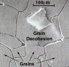
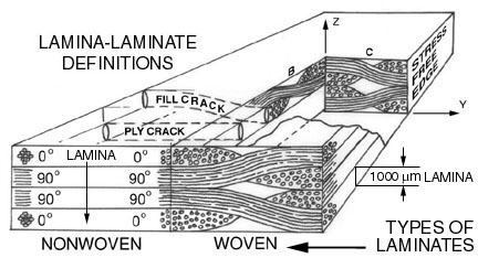
Figure 1. Microstructures of grains and lamina
Ronald D. Kriz, Associate Professor
Engineering Science and Mechanics
Virginia Polytechnic Institute and State University
Blacksburg, Virginia 24061


Macroscopic mechanical behavior can be influenced by structures at the microscopic scales of 10-3m. For example elastic properties of a polycrystalline material are controlled by the orientation of individual grains sizes of 10 -3m, i.e. random orientation leads to isotropic macroscopic elastic properties. For composite laminates macroscopic properties of laminated composites are influenced by the elastic properties and fiber orientation in each laminate layer ("lamina"). Typical lamina thicknesses are 10-3m and hence are considered microscopic structures. Cumulative damage events, i.e. ply cracks, at the lamina-microscopic scale can also influence mechanical behavior and failure at the macroscopic laminate scale. Relationships between the microscopic and macroscopic scales embraces a wide variety of other topics and examples. It is not the intention of this section to provide a comprehensive overview of these micro/macro models but rather to introduce the students to examples of micro/macro models that is representative of the research conducted by Dr. Ron Kriz while working with computers at NIST (formerly NBS) from 1980 to 1990 and with computers at NCSA (National Center for Supercomputing Applications) from 1990 to 2000. During this time period high performance computing was rapidly evolving. CDC, Thinking Machine CM2, Cray, and SGI computers were all used to study the mechanical behavior of a variety of problems related to damage in laminated composites and wave propagation in highly anisotropic crystals and fiber-reinforced composites.
Throughout this section we provide links to examples where the reader can work with interactive computer programs, written by Dr. Kriz, as they relate to the theory developed in the sections below. Hence our objective is to create an interactive section that compliments the theory and allows the student to experiment with the various micro/macro models as they are introduced.
Cracks span the scales. The mechanical behavior of materials with cracks can
be modeled to include: 1) the influence of individual atoms ("nano"), 2) the presence of
interfacial layers separating different microstructures ("micro"), or 3) the idealized
continuum model where atomic and interfacial effects are neglected ("macro").
Regardless of the scale, models make simplifying approximations. Understanding these
approximations is key to understanding how some models bridge the scales. Therefore
we will highlight these approximations below as we develope the theory and also when
we develope the mathematical model for each of the scales. The images on the home page
exemplify these three scales.
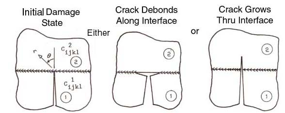
In this section we focus our attention on modeling the mechanical behavior of
materials that are influenced by cracks at or near interfacial layers or grain
boundaries. The image in the center of Fig. 2 shows a schematic of a crack
that has intersected a boundary between two dissimilar materials: region 1 and
region 2. This boundary can be a grain boundary or interfacial layer separating
two different lamina in a composite laminate. In either case the model for
predicting the behavior of crack propagation is fundamentally the same but in
the following sections we will focus mostly on interfaces in laminated composites.
Numerous models for interfacial cracks exist. In the most general case we assume a crack
arrested at an interface separating two dissimilar anisotropic materials and then simplify
the model to dissimilar isotropic materials. Such cracks are common in fiber-reinforced
composite laminates. In Figure 3 we show a schematic and an acetate replica micro-graph of a 90 degree
ply crack arrested at a 0/90 degree ply interface.
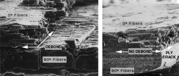
If the crack continues to propagate, it can grow into the adjacent 0o ply, causing
the fibers to fail or it can grow into an interfacial crack and debond along the 0/90 interface.
Figure 4 shows experimental evidence of both types of crack growth, that can be controlled
by the residual stress state, Ref.[1].
Statistical evidence
confirms that laminate fracture strength is lower, if the ply crack extends into the 0o load bearing ply, and higher if the ply crack extends along the interface as an interfacial debond. Hence we
have experimental evidence that macroscopic laminate fracture strength is controlled by
damage at the microscopic lamina scale.
With this experimental evidence the problem at hand is to create a model that will scale both the micro and macro and predict crack growth near an interface between two dissimilar materials. With such a model we can then study which parameters control crack growth. Does the residual stress state, anisotropy, or both control how the crack grows near an interface? The most general mathematical formulation is shown in Figure 5.
From elementary fracture mechanics we can idealize the singular stresses near the ply crack
tip as a linear superposition of Mode-I, Mode-II, Mode-III stress states. The superscripts
and subscripts I, II, and III represent the three different fracture Modes. The exponent
-α on the variable "r" (radius) has a value of -1/2 for isotropic and homogeneous
anisotropic materials, but differs from -1/2 for dissimilar isotropic materials, which
will be discussed below. The constants CI, CII, and
CIII are functions of Stress Intensity and radius "r", and the variables
FijI, FijII, and
FijIII are functions of geometry only, i.e. location of
boundaries and the angle, θ, measured at the crack tip. The
remainder of this section will focus on deriving simple relationships for the special case of
two dissimilar isotropic regions. After we learn more about anisotropy we will return to this
problem where the dissimilar regions are anisotropic.
An introduction of the different fracture Modes is provided in classic fracture mechanics publications, Ref.[2,3] and at the Department of Materials Science and Engineering (MSE)
Fracture Web Site (Student Team Project MSE2094, Spring 1997), see section on
"Energy Methods
" and "Stress Intensity"for an introduction to the different fracture Modes.
The first model of a crack near interfaces separating dissimilar isotropic materials was developed by Williams Ref.[4,5].
Williams Ref.[4] was the first to show that the singularity on "r" for an interfacial crack, "Debond" between two dissimilar materials, exhibited an oscillating singularity.
Derivation of this equation will be outlined and discussed in class. Although
the solution is correct mathematically, the strong oscillation predicted as the
observer approaches the crack tip is physically unrealistic. Research by Dan Post,
Professor at Virginia Tech, experimentally confirm a stress reversal near a
debond crack by high resolution Moire Interferometry but although this is an
encouraging piece of information it is far from what we need to confirm a full
oscillation. Whether or not such a oscillating singularity can exist in a real
material and at what scale such an oscillation might exist is exactly the type
of question that arises when we try to interpret and justify model predictions.
Although we are at the micro level were the crack behavior is controlled by two
"thin" dissimilar isotropic materials we still assume a continuum but this
approximation breaks down as we approach atomic spacing ("nano"). Are such
oscillating singularities a realistic mechanical behavior that can be modeled at
the nano scale? Probably not. At this point this type of behavior is at best only
an interesting mathematical solution to a interfacial debond solution at the
microscale that suggests that this behavior extends into the nanoscale -- maybe.
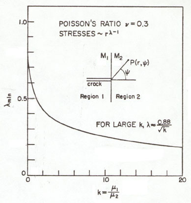
Williams Ref.[5] also showed that the singularity for a crack acting normal to an interface
between two dissimilar isotropic regions is a function of the ratio of the elastic shear moduli
of these two regions. Here we derive an expression for the exponent, λ on the radius
"r". The exponent, λ is calculated as an eigenvalue or root from the characteristic
equation below.
In the early part of the 20th century most engineering materials were isotropic.
In the later part of the 20th century, 1970s -> 1990s, the aerospace industry
created the demand for new, high-strength, high stiffness and light-weight
fiber-reinforced composite materials. Because these materials are also highly
anisotropic, designers could optimize their designs, i.e. orient the direction of
high stiffness and strength in the load direction. Other materials used in "Smart"
or "Intelligent" structures, such as piezioelectric polymers are also highly
anisotropic. Because the properties of these new materials could be tailored,
designers, could for the first time, design the material for the application
instead of designing an application around fixed material properties.
Anisotropic materials are becoming the material of choice in a variety of
engineering applications as we enter the 21st century. Studying the mechanical
behavior of these highly anisotropic materials under static and dynamic loads at
all scales is relevant when considering current engineering practice.
In the early part of the 20th century anisotropy was more a topic of scientific
research then a property used in engineering design. Nye's text on "Physical
Properties of Crystal", Ref.[6], gives an excellent introduction to anisotropy in
crystals from a material scientist perspective. Lekhnitski's text on "Theory of
Elasticity of an Anisotropic Body", Ref.[7], began to address issues of anisotropy
in engineering design. In this section we will give a very brief introduction to
anisotropy for a continuum (macroscale) and then apply what we learned to
anisotropic laminates at the microscale. In section 10.0 we will also show how
anisotropy can significantly control dynamic mechanical behavior in a continuum
(macroscale).
Mechanical behavior of anisotropic materials is characterized in the most general
notation as a fourth order stiffness tensor, Cijkl, which is contracted
into a six by six stiffness matrix, Cα,β, relating six
components, σα, of a symmetric stress tensor to the six
components, eβ, of the symmetric strain tensor which are
written here as column vectors.
Although this contracted notation shown above is convenient and will be used below
to model mechanical behavior of anisotropic laminates at the microscale, a more
complete description of elastic anisotropy will require that we return to the more
general form where the stiffness matrix that relates strains to stress is written
as a fourth order stiffness tensor Cijkl, where the stresses,
σij, and Lagrangian strains,
lij, must then be written as
second order tensors. We will show that this more general tensoral form will
allow us to create unique three dimensional geometric representation surfaces for
each unique anisotropic elastic symmetry.
First we will show how stress can be written in the form of a second order tensor.
The proof that stress is a second order tensor because it transforms as a second
order tensor is given in Ref.[8].
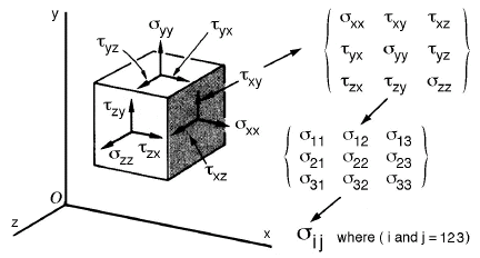
Figure 7 shows how all possible components of stress acting as forces on a small
differential element can be organized into a matrix format which can also be
reduced to index notation where i and j are called "free" indices that are assigned
values of 1, 2, or 3. All possible combinations of the i and j indices yield the
desired three by three matrix.
Figure 7. Stress tensor components shown on a differential element
Writing all six components of strain into a similar matrix is not as straight
forward as it was for stress where each stress components could be simply seen
as a force acting on the surface of a cube. Strain implies displacement which
requires much more development, see Ref.[8] Chapter 3, "Analysis of Deformation
in a Continuum". Suffice it to say that strain like stress has 9 components
which can be identified with the same indices which identifies a displacement
direction or shearing in a plane associated with each strain component. From a
Lagrangian viewpoint, for large displacement gradients, the nonlinear strain
displacement relationships are shown below.
If we assume only small displacement gradients then the nonlinear terms can
be neglected and the upper case "L" is reduced to the lower case "l"
which is used to denote the linear lagrangian strain tensor,
lij.
With strain and stress defined as second order tensors, it is not difficult
to derive the desired linear anisotropic relationship, equation (5), from the
first law of thermodynamics. One form of the first law of thermodynamics is
shown below.
where u is the specific internal energy per unit mass, ρ is the density,
eij is the Eulerian strain associated with Eulerian displacement
gradients, c is the radiative heat transfer per unit time per unit mass,
and bi is the heat transferred through a unit surface per unit
time. Note d/dt is the total or comoving derivative. For a complete derivation
see Ref.[8], Chapter 4, section 4.5.
If we assume no heat transfer by radiation or conduction and we assume that
only small displacement gradients result in lagrangian strains,
lij, equation (8) reduces to a form where u is now called
the strain energy per unit mass since the only mechanism available for storing
internal energy in the continuum is through deformation.
Next let's assume density is constant, or at least a function of strains and that
stresses are related to strains by some unknown function (to be determined). Hence
strain energy can be a function of stress or strain. For the purpose of discussion
here we assume strain energy can be written as some function of strain.
Substituting equation (11) into equation (9) yields.
If this relationship is true for any arbitrary nonzero dlij, then
the relationship in the parenthesis must vanish which yields an equation that
shows the relationship between stress, strain and strain energy per unit mass.
Recall that for equation (10) we assumed some undefined functional form for
strain energy as a function of strain. One possible function would be to
expand the strain energy into a power series whose coefficients like strain
are tensors but constants with indices that sum ("contraction") with the indices
of the strain tensors such that each term in the series is a scalar component
of the strain energy. The first term α is an
arbitrary energy reference state, so we can set it to zero. The second term
is a zero strain reference state. The third term is the linear elastic term
and the fourth term is the nonlinear, but elastic, term. Higher order terms
can be added here as needed to model the desired constitutive stress-strain
relationship.
Substituting this function for strain energy into equation (13) yields the most
general form of the anisotropic elastic constitutive law in tensor format.
NOTE: 1) it is perhaps more evident at this point that the coefficient
βij represent the residual stresses when
the strains, lij, go to zero, and 2) the coefficient
δijklmn is the nonlinear elastic term that gives
rise to nonlinear elastic stress-strain diagrams not associated
with dissipative constitutive models, which we also set to zero. With these
simplifications equation (15) reduces to the desired linear-elastic equation.
Where Cijkl are the terms that relate components of strain to the
components of stress per unit mass. A similar expression without density can
be derived where strain energy per unit volume is introduced into the derivation.
Interestingly to remove density is not as straight forward as one might think,
see Ref.[8].
Lets briefly look at an arbitrary geometric transformation of equation (17). For a
full development of this type of transformation see Ref.[8]. It can be shown that
both stress and strain are second order tensors because they transform as second
order tensors and Cijkl transforms as a fourth order tensor.
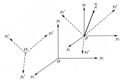
Figure 8. Vector drawn with respect to two different Cartesian axes
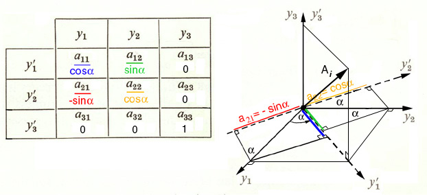
Introduce the direction cosines between the two sets of axes:
Figure 9. Direction Cosine Matrix With a Simple Rotation About the y3 axis.
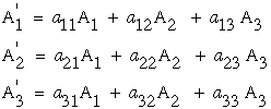
Hence, the relation between the vector A' and A can be
summarized as follows.
Note that the indices on A' can be replace as i=1,2,3 hence the three
equations in equation (21) reduces to one equation with a "free" index "i".
Also note that when the number in each term in equation (22) are the same (1 1 in
the first term, + 2 2 in the second term, and + 3 3 in the third term) we
introduce a new idea of a "summation" notation where any such summation can be
notationally simplified and replaced with repeated indices in one term. Hence
we can now use this summation index to reduce equation (22).
The same direction cosine matrix, aij, can also be used in the
transformation of stress, strain, and stiffness, in equations (18), (19),
and (20) which when substituted into equation (17) reveals that the same
equation exists in the arbitrary prime coordinate system, equation (24).
The fact that equations (17) and (24) are identical demonstrates that
equation (17) is invariant to any ARBITRARY transformation, hence
equation (17) is a "tensor equation". The keyword here is arbitrary.
Equations (17) and (24) are the form of Hooke's Law we need to continue
the discussion of anisotropic elasticity by Nye and also to show some
interesting "glyphs" (geometric representations) of the fourth order
stiffness tensor, Cijkl .
Now that we have introduced elastic anisotropy both as a fourth order tensor
and a six-by-six matrix with reduced notation, the reader can now
understand the comprehensive treatment of elastic anisotropy given by
Nye, Ref.[6], in chapter 8, "Elasticity. Fourth-Rank Tensors", pp. 131-149,
where both stiffnesses and compliances are described in terms of matrix and
tensor notation. Our objective here is to summarize and highlight the
different elastic anisotropies commonly encountered by todays materials
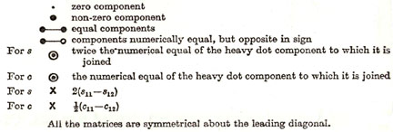
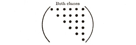
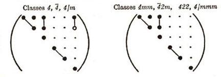
engineers. Figure 10 summarizes the various elastic anisotropies in matrix notation.
Figure 10. Various anisotropies for Sij and Cij.
As shown in Figure 10, the different elastic anisotropies are related to
the number of independent terms in the elastic property matrix where
symbols represent either stiffnesses or compliances. Each of these unique
matrices can be related to crystal symmetry classes but here we will
discuss just a few of the major classes and symmetry conditions. Triclinic
is the most general with 21 independent components. Starting with Triclinic
the number of independent terms can be reduced using symmetry planes and
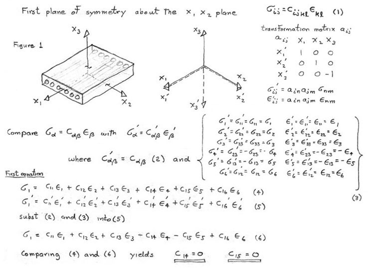
invariant rotations. For example if we could imagine ourselves standing
inside a crystal and observed that the crystal structure looked identical
if we looked either in the +z or -z direction. With this observation we
would conclude that symmetry exists about the x-y (1-2) plane and the
transformation matrix, aij, would be the identity matrix but
with the term a33 set equal to -1, see Figure 11. Using this
transformation matrix in equation (17) components of the stress tensor
are compared in the primed and unprimed coordinates.
Figure 11. Sample calculation of transformation for symmetry about
the x-y (1-2) plane.
This comparison determines which matrix terms must vanish. For example
in Figure 11 comparing σ1 with
σ1' requires C14
and C15 vanish. Similar comparisons with the other stress
components requires,
Hence this reduces the Triclinic with 21 independent terms to Monoclinic with
13 independent terms. Figure 10 shows two different types of Monoclinic
matrices. If we continue with symmetry in the x-z and y-z plane additional
terms must vanish and Monoclinic reduces to Orthotropic with 9 independent
terms. Arbitrary rotation about the z axis (3-direction) assuming elastic
properties are invariant reduces Orthorhombic to Hexagonal with five
independent terms. Of course for isotropic there are only two independent
terms or components of the stiffness or compliance fourth order tensor.
Elastic symmetries commonly encountered when working with fiber-reinforced
materials commonly used in lightweight aircraft and aerospace structures, are
called "orthotropic" which is the same as orthorhombic and "transversely
isotropic" which is equivalent to hexagonal.
We continue the development of anisotropic mechanical behavior into two
sections. First we focus on engineering elastic properties and represent
anisotropy in terms of engineering properties: E, G, and ν, and second
we focus on all components of the fourth order stiffness
tensor. In both cases we ephasize the use of geometry to study the
anisotropy.
Another linear constitutive relationship, similar to equation (24), exists
for compliances, Sijkl, that relate stresses with strains.
Compliances like stiffnesses can be considered fourth order tensors because
they transform as fourth order tensors.
Hence the relationship between compliances and stiffness can be shown as
an inverse relationship. This inverse relationship is shown here in
reduced contracted notation. NOTE: although these matrices are inversely
related, Sij and Cij are not tensors quantities
because they do not transform as second order tensors.
Compliances, unlike stiffnesses, have a simple relationship with engineering
elastic properties such as Young's modulus, shear modulus, and Poisson's ratio.
For example the compliance along the z axis (3-direction), S33 is
defined as the reciprocal of the Young's modulus in the same z-direction.
Similarly expressions for shear modulus and Poisson's ratio in the y-z (2-3)
plane can be simply derived from terms in the compliance matrix.
It is now possible to show how these three engineering elastic properties
vary as a function of rotation from the z axes (3-direction) into the x-y
(1-2) plane by using the general fourth order compliance tensor transformation
of equation (27) where the direction cosine terms, aij, are
expanded into sines and cosines of the rotation angle,
θ, starting at zero along the z axis and rotating 90o into
the x-y plane. This transformation although simply done as a fourth order
transformation, becomes a tedious task in reduced contracted notation. After
much algebra the final equations are simplified, see Ref.[9].
For all isotropic engineering materials equations (32), (33), and (34) will, by
definition, reveal no variation in properties as we rotate from the z axis into
the x-y plane, hence circles in a two-dimensional (2-D) plane or spheres in a
three-dimensional (3-D) space are visual representations (manifestations) of
isotropic elastic properties. Unidirectional fiber-reinforced composite materials,
on the other hand, exhibit highly anisotropic behavior which is exhibited as
significant deviations from the isotropic spherical geometry.
2.0 Cracks: Atomistic 10-9m - at Interfaces 10-3m - in a Continuum 100m
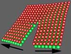
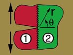
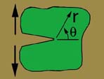
Figure 2. Schematic of Mode-I cracks spanning the length scales
3.0 Cracks Near Interfaces Between Dissimilar Isotropic Materials


(1)

(2)

(3)
4.1 Introduction to Mechanical Behavior of Anisotropic Materials
Our previous discussion on laminated structures provides many microscale examples
of mechanical behavior. Since most composite laminates are highly anisotropic it
would be appropriate to first learn more about how anisotropy influences
mechanical behavior and then we can proceed with an introduction to the mechanical
behavior of anisotropic laminates.

(4)

(5)

(6)

(7)

(8)

(9)

(10)

(11)

(12)

(13)

(14)

(15)

(16)

(17)

(18)

(19)

(20)
Transformation Law of a vector
(21)

(22)

(23)

(24)
KEY TO NOTATION
TRICLINIC (21)
MONOCLINIC (13)

ORTHORHOMBIC (9)
CUBIC (3)

(7) TETRAGONAL
(6)
(7) TRIGONAL
(6)

HEXAGONAL (5)
ISOTROPIC (2)

NOTE: transformation of stress and strain requires the
use of tensor transformations
eqns. (18) and (19) to get the correct sign.

(25)

(26)

(27)

(28)

(29)
 ,
, 
(30), (31)

(32)

(33)

(34)
| Material | C33 | C11 | C12 | C13 | C44 | ν32 | ν12 |
|---|---|---|---|---|---|---|---|
| Epoxy-matrix (Kriz-Stinchcomb, 1979) | 8.63 | 8.63 | 4.73 | 4.73 | 1.95 | 0.345 | 0.345 |
| Carbon-fiber (Kriz-Stinchcomb, 1979) | 235 | 20.0 | 9.98 | 6.45 | 24.0 | 0.279 | 0.490 |
| Carbon-fiber (Dean-Truner, 1973) | 240 | 20.4 | 9.40 | 10.5 | 24.0 | 0.35 | 0.497 |
| Carbon-fiber (Smith, 1972) | 221 | 19.4 | 6.60 | 5.80 | 20.3 | 0.230 | 0.320 |
| Composite (60% Fiber) (Kriz-Stinchcomb), 1979) | 144 | 13.6 | 7.0 | 5.47 | 6.01 | 0.284 | 0.497 |
| Material |
Poisson's Ratio(ν)
Modulus: Bulk(K), Shear(G), Young's(E) Subscripts: Matrix(m), Fiber-Axis(L), Transverse-Plane(T) |
||||
|---|---|---|---|---|---|
| Isotropic: two independent properties-> | Em | νm | |||
| Epoxy-matrix (Kriz-Stinchcomb, 1979) | 5.35 | 0.345 | |||
| Hexagonal: five independent properties-> | EL | ET | GLT | GTT | KTT |
| Carbon-fiber (Kriz-Stinchcomb, 1979) | 232 | 15.0 | 24.0 | 5.02 | 15.0 |
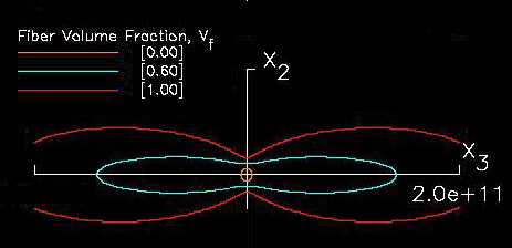
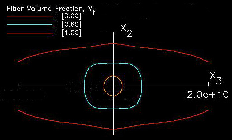
For example if we take elastic properties predicted in Ref.[10], see Table 1., for unidirectional carbon-fiber/epoxy composites and substitute these properties into equations (32), (33), and (34), both spherical and nonspherical geometries are predicted, see Figures 12, 13, and 14. In these figures the elastic properties are also shown as a function of fiber volume fraction where 0.0 fiber volume fraction yields pure isotropic epoxy properties, shown as circles, and 1.0 fiber volume yields pure anisotropic fiber properties and hence the geometry significantly deviates from the circular geometry. Even low fiber volume fractions yield significant anisotropy.
Click on image to start an interactive JWave session
Click on image to start an interactive JWave session
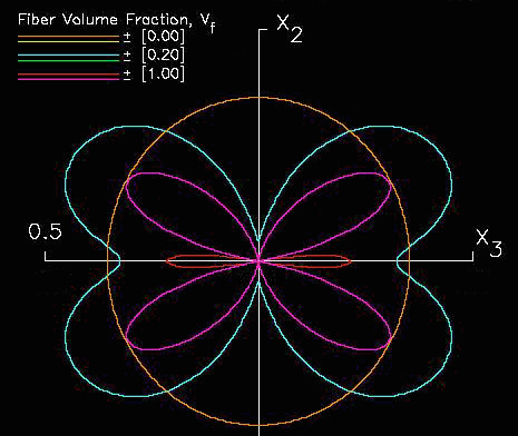
Figure 14. Polar diagram of graphite/epoxy Poisson's modulus ν32
for various fiber volume fractions, in GPa.
NOTE: yellow, green, and purple line indicates negative Poisson's ratio.
A closer look at these figures reveals some obvious facts, but also some unexpected new information. If all fibers are aligned along the z axis (3-direction) then we would expect that the elastic stiffness would be largest along the z axis (3-direction) and less stiff in the x-y (1-2) plane. Indeed this trend is confirmed geometrically. However unexpected properties are observed such as a large negative (-0.354) Poisson's ratio, see purple line in Figure 14. A negative Poisson's ratio would require that the material would expand both in the load direction and transverse direction to the load direction. If the material is transversely isotropic the transverse expansion would be the same in all directions within the transverse plane. Putting this all together would require that such a material when loaded in the fiber direction would expand in all directions, hence it's volume would increase under a uniaxial tension load.
Perhaps the reader might find other interesting mechanical behavior by experimenting with either the links to "Interactive JWave session" shown above each of the figures (12,13,14), or below an alternate link is provided that provides the student access to a more comprehensive interactive session with access to: (1) computer programs, (2) sample data files, (3) numerical results, and (4) images.
The elastic properties: Young's Modulus, E, shear modulus, G, and Poisson's Ratio, ν, in each orthogonal plane can be used to classify the nine independent orthorhombic elastic constants in terms of engineering properties.
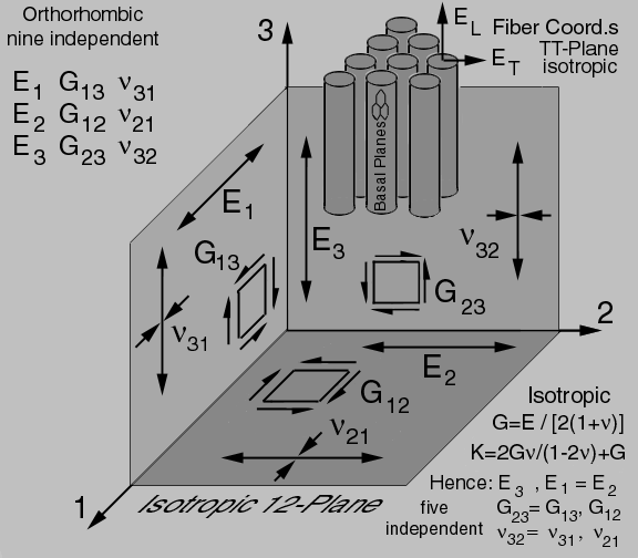
Figure 15. Transversely-isotropic carbon fibers and their composites.
With the mechanical behavior ("deformation") shown in each plane of Fig. 15 it is easier to see how each of these nine properties are independent. If all the fibers are aligned along the 3-axis, it is easy to see the 12-plane is transversely isotropic and the number of independent elastic properties reduce to 5 (hexagonal symmetry) and the isotropic relationships can be used in the 12-plane. The large negative Poisson's ratios predicted in Fig. 14 is most likely due to the nano-structure of the graphite fibers where basal planes become aligned parallel to the circumference when pyrolyzed. This pyrolyzation also creates a lamellar structure of basal planes aligned parallel to the fiber longitudinal axis ("L") and explains the unusually high elastic stiffness along the x3 axis. Together these two nano-structural observations explain the fiber has transversely- isotropic ("hexagonal") symmetry. Here we choose the fibers longitudinal axis to be parallel to the x3 axis because for hexagonal symmetry the x3 axis is the conventional "unique" symmetry axis. However in engineering design the x1 axis is choosen as the fiber-axis convention.
A brief literature review has revealed some interested hypothetical structures for pyrolyzed carbon fiber structures, see Figure 16. Although preliminary observations can explain how this nano-structure results in a large modulus along longitudinal fiber axis, much more research needs to be done before we can conclude any nano-structure property relationship that can explain the large negative Poisson's ratios.
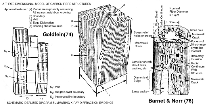
Figure 16. Carbon fiber pyrolyzed structures Ref.[11] and Ref.[12].
Because so little is known about these transversely isotropic ("hexagonal") fiber properties, engineering designers make some gross approximations. For example the five independent elastic properties shown in Fig. 15 are further reduced to four independent elastic properties by equating all three shear moduli and similarly all three Poisson's ratios are also equated.
These same fiber-reinforced materials and their peculiar anisotropies will be used in the next section on "Laminated Plate Theory". As a result we can expect some unusual mechanical behavior of laminated plates fabricated with these materials at the micro level.
Geometric representations of engineering elastic properties, E, G, ν, although interesting, can only reveal variations of just that one property. The modulus E3 = S33-1 represents only one of nine components of a fourth order tensor and consequently does not represent the full anisotropy of all components of the stiffness tensor. Next we will show how to geometrically represent anisotropy that includes all possible terms (components) of the fourth order stiffness tensor.
To include all components of a fourth order stiffness tensor in a geometric representation of anisotropy requires we look closer at the equations of motion for an anisotropic solid (dynamic mechanical behavior). Here our objective is to look at a spherical disturbance such as a dilitational pulse that expands equally in all directions: invoking Huygen's principal the reader can envision a very small plane wave exists on the surface of a very small sphere in the center of an anisotropic crystal. One can simply imagine that from Huygen's principal each of these plane waves travels in a specific direction, direction cosines, νi, at a speed that corresponds to elastic properties unique to the same direction. Hence, plane waves traveling in different directions will travel at different speeds and the continuous collection of all of these plane waves, although initially a sphere, soon deviates into a nonspherical shape simply because plane waves will travel faster in stiffer directions and slower in less stiff directions. This idea was modeled and simulated for a highly anisotropic Calcium-Formate crystal, "Spherical Wave Simulation in 2-D Anisotropic Media". The three-dimensional wave surface for a Calcium-Formate crystal was first plotted in Ref.[13]. We will show that this wave surface topology does indeed uniquely describe the complete set of components of the fourth order stiffness tensor. These resulting geometries are now being used as new sub-classification schemes within orthorhombic symmetry, Ref.[14].
First we start with the equations of motion for a continuum.
 |
(35) |
Recall equation (17)
 |
(17) |
and substitute the strain-displacement relationship, equation (7),
 |
(7) |
into equation (17) yields
 |
(36) |
Recall that the strain tensor is symmetric which further reduces equation (36).
 |
(37) |
Substitituting equation (37) into equation (35) yields the equation of motion in terms of displacements.
 |
(38) |
This equation can be further reduced if we assume the material is homogeneous.
 |
(39) |
With this simplification equation (38) reduces to a form where we can now assume a solution for displacement and substitute it into this equation.
 |
(40) |
Let us assume a small plane wave periodic disturbance, see Figure 17.
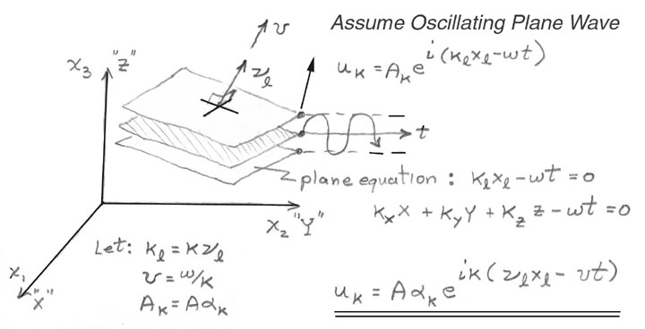
Figure 17. Mathematical model for a plane wave disturbance: oscillating plane written in exponential format in terms of wave velocity, v, propagation direction, νl, and particle vibration direction, αk
The periodic displacement shown in Figure 17 uses an exponential functional form instead of sines and cosines because it will be easier to differentiate. The reader can envision a plane wave in Figure 17 where the wave number coefficients, ki, are terms used to define a plane (this will perhaps require a review of basic descriptive geometry in freshman calculus) and the circular frequency, ω, when multiplied by time, t, replaces the constant for a plane with a term which models the oscillatory motion of that plane.
 |
(41) |
The terms in equation (41) can be replaced with wave velocity, v, and direction cosines of the propagation direction, νi which will allow the reader to interpret the results of this particular eigen-problem in a more meaningful way.
 |
(42) |
Substituting equation (42) into equation (40) and after much manipulation, equation (40) reduces to an eigen-value problem which is written below in both tensor and matrix notation.
| tensor equation: |
 |
(43) |
matrix equation:
 |
(43) |
If we use the matrix form of equation (43) it is easier to see that the velocity terms along the diagonal, ρv2, are the eigen-values and the displacement direction cosines, αi are the eigen-vectors. Closer examination of the solution to this particular eigen-value problem reveals that both the eigen-values and eigen-vectors can only be functions of ALL stiffness tensor components for an assigned propagation direction, νi. Hence we conclude that if we solve for eigen-values (wave speeds) in all possible propagation directions, νi, and connect points to form a continuous surface, this would generate a 3-D shape of wave speed for each eigenvalue. Since there are three eigen-values, equation (43) predicts three wave surfaces: 1) longitudinal which is usually the fastest and observed as the largest shapes, and 2) two different shear ("transverse") waves which are usually slower and consequently observed as smaller shapes. The eigen-vectors which are particle vibration direction cosines (0 to 90 degrees) can be mapped onto the eigen-value surfaces as color. Hence the color would reveal the type of wave: longitudinal (0-degrees i.e. purple) and transverse (90-degrees i.e. red) where green would indicate a mode transition from longitudinal to transverse. With colors the observer can quickly determine the wave type and discover possible mode transitions. Graphical definitions of these and other properties associated with this solution are given by the problem statement / updated statement.
Some obvious geometric features that correspond to anisotropy are: 1) stiffer directions map as a larger distance from the geometric center which would be seen as "bulges" and 2) less stiff directions map as smaller distances from the geometric center which would be seen as "depressions". Highly anisotropic materials would appear as significantly deviating from the isotropic spherical geometry. Graphite-Epoxy and Calcium-Formate exemplifies all of these features, see Figure 18 and Figure 19.
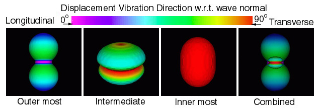
Figure 18. Wave surfaces predicted for Graphite-Epoxy, Hexagonal symmetry
NOTE: light-blue/green indicates a mode transition -- a very rare anisotropy
which
is only observed in Calcium-Formate, spruce-wood, and graphite/epoxy.
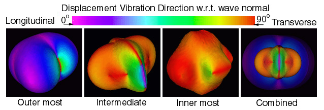
Figure 19. Wave surfaces predicted for Calcium-Formate, orthorhombic symmetry
NOTE: light-blue/green indicates a mode transition -- a very rare anisotropy
which
is only observed in Calcium-Formate, spruce-wood, and graphite/epoxy.
Figure 19 shows the solution of equation (43) for an orthorhombic fourth order stiffness tensor of Calcium-Formate, Ref.[13]. This particular tensor has a rare anisotropy that requires all three wave surfaces to connect into a single contiguous surface, see "combined" wave surface of Figure 19. A simple movie demonstrates both the connected surfaces and mode transitions previously described. The only other known material that exhibits this anisotropy (geometry) is Spruce wood. References [13-15] identify four possible geometries not previously known. With these geometries it is now possible to derive a subclassification scheme for orthorhombic anisotropy.
By studying the wave surface geometries it is also possible to study and compare elastic property anisotropy from isotropic to orthorhombic symmetry. Below is a table listing elastic material properties for each of these symmetries.
| Material: Stiffnesses GPa | Density gm/cm3 |
C11 | C22 | C33 | C44 | C55 | C66 | C12 | C13 | C23 |
|---|---|---|---|---|---|---|---|---|---|---|
| Stainless Steel (isotropic) / Update | 7.88 | 261.0 | 261.0 | 261.0 | 77.5 | 77.5 | 77.5 | 106.0 | 106.0 | 106.0 |
| Aluminum, (cubic) / Update | 2.7 | 108.0 | 108.0 | 108.0 | 28.0 | 28.0 | 28.0 | 62.0 | 62.0 | 62.0 |
| Zinc (hexagonal) / Update | 7.10 | 143.0 | 143.0 | 50.0 | 40.0 | 40.0 | 63.0 | 17.0 | 33.0 | 33.0 |
| Aligned Graphite/Epoxy (hexagonal) / Update | 1.61 | 14.5 | 14.5 | 160.0 | 7.07 | 7.07 | 3.62 | 7.26 | 5.53 | 5.53 |
| Tellurium Oxide (tetragonal) / Update | 4.99 | 55.7 | 55.7 | 106.0 | 26.5 | 26.5 | 65.9 | 51.2 | 21.8 | 21.8 |
|
Benzene (orthorhomibic Type-1)
/
Update
( C11, C22, C33 ) > ( C44, C55, C66 ) |
1.06 | 6.14 | 6.56 | 5.83 | 1.97 | 3.78 | 1.53 | 3.52 | 4.01 | 3.90 |
|
Calcium Formate (orthorhombic Type-2)
/
Update
( C11> C33> C 66> C22> C55> C 44 ) |
2.02 | 49.2 | 24.4 | 35.4 | 10.5 | 12.2 | 28.2 | 24.8 | 24.5 | 14.5 |
|
Hypothetical (orthorhombic Type-3)
/
Update
( C11> C66> C55> C22> C44> C33 ) |
6.00 | 180.0 | 45.2 | 10.3 | 20.4 | 45.5 | 90.6 | 0.100 | 0.200 | 0.300 |
|
Hypothetical (orthorhombic Type-4)
/
Update
( C11> C22> C66> C44> C55> C33 ) |
3.00 | 80.1 | 60.2 | 10.3 | 30.4 | 20.5 | 40.6 | 0.100 | 0.200 | 0.300 |
Figures below correspond to the last four orthorhombic symmetries and their corresponding elastic property inequality.

Figure 20. Examples of the four basic types of geometries and their corresponding
inequalities that can be used to subclassify within orthorhombic symmetry
The inequalities for each of the four types of orthorhombic symmetries are the necessary and sufficient condition that defines each unique geometry. These geometries and their corresponding inequalities can be used to create a subclassification scheme within orthorhombic symmetry. For those interested we have provided a graphical proof.
Other highly anisotropic materials such as graphite/epoxy can also significantly influence dynamic mechanical behavior. The section on Simulation and visualization of wave propagation in unidirectional graphite/epoxy composites Ref.s [16], [17], and [18], summarizes how unidirectional graphite/epoxy composites like Calcium Formate exhibit mode transitions but without resulting in a connected wave surface. Unlike Calcium Formate, which is a crystal, graphite/epoxy derives its anisotropy from its' constituent fiber and matrix properties (microscale), hence elastic properties at the microscale can signficantly influence anisotropy and dynamic mechanical behavior at the macroscale. For graphite/epoxy it can be shown that not only can anisotropy have a significant effect on dynamic mechanical behavior, see Figure 21, but degradation of either the fiber or matrix phase can preferentially alter the direction of the wave propagation from the initial undegraded state, see Figure 22. A section on simulation-visualization in unidirectional graphite/epoxy composites allows the reader to explore the influence of anisotropy on these and other possible dynamic mechanical behaviors using a small grid (30x60) or large grid (45x180) finite element grid model. For confirmation with an exact solution a simple isotropic one-dimensional model is provided here for the reader. Experimental confirmation of the accuracy of these physical based simulation models is given in Ref.[10] Figure 14, see Figure 23.
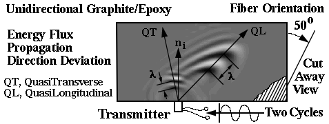
Figure 21. Schematic of simulation and
animation
summarizing
wave properties of a full field simulation.

Figure 22. Influence of preferential microscale elastic component
degragation on macroscale mechanical behavior.
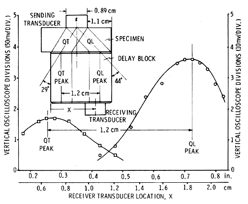
Figure 23. Experimental confirmation of beam steering, Ref.[10] Figure 14.
The discussion above provides an excellent example of how elastic properties scale from the nanoscale (fiber transversely-isotropic nano-structure) to the microscale (transversley-isotropic unidirectional composite) and ultimately influence the dynamic mechanical behavior at the macroscale (beam steering and mode transitions). The diagram below illustrates how the wave length of a stress wave scales from the macro to the nano structures. Indeed the commponents of the elastic stiffness tensor are derived from the nanostructure of the atomic spacing.
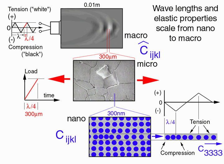
Figure 24. Wave length and elastic properties scale from nano to macro.
Other sections on: 1) Visualization of Stress Waves in Elastic Solids and 2) Simulation and Visualization of Energy Waves Propagating in 2-D and 3-D Anisotropic Media, provide more information on how anisotropy controls dynamic mechanical behavior.
We have demonstrated that anisotropy in crystals like Calcium-Formate and undirectional composites like graphite/epoxy exhibit unusual dynamic and static mechanical behavior. As designers we can take advantage of this anisotropy. Because the elastic properties of graphite/epoxy can be tailored, engineers can design the material for the application instead of designing an application around fixed material properties. One popular method of exploiting the anisotropy of graphite/epoxy, in the design of a desired mechanical behavior, is to use laminate plate theory.
In the previous section, 4.1 Introduction to Mechanical Behavior of Anisotropic
Materials, mechanical behavior of individual anisotropic layers, "lamina", of
the "laminated" plate can now be used to model the mechanical behavior of the
laminate. The purpose of this section is to introduce the reader to the basic
ideas of laminated plate theory so that the reader gains an understanding of
the relationship between the two scales. To gain a working knowledge of
laminated plate theory, we encourage students to take ESM4044 MECHANICS OF
COMPOSITE MATERIALS and ESM6104 MECHANICS OF COMPOSITE STRENGTH AND LIFE .
With a working knowledge of laminate plate theory, designers can taylor the
elastic properties and orientation of each lamina, hence optimize their design
by controlling the properties and orientations of each lamina. At the end of
this section we will outline several examples on how the mechanical response
of a laminated plate can be controlled ("designed") by lamina properties, but
first we briefly outline the derivation of the analytic model needed to
understand how properties at the microscale control mechanical behavior at
the macroscale.
Analytic Model:
Consider an orthorhombic lamina in plane stress and let the 1-2 axes shown in
Figure 26 be aligned with the fiber axis. In plane stress we assume the lamina
is very thin and the stress through the lamina thickness is very small.
The elements of [Q] are related to the engineering constants E,G, and
ν as follows
Transformation of lamina stress and strain from the 1-2 axes to the
rotated x-y axes is shown here in matrix notation. This transformation
is different from the transformation for all components of the second
order tensor because here we have only three components of stress and
strain because of the plane-stress condition.
where
The lamina stress-strain relationship in the rotated x-y coordinates
In reduced matrix notation
where
The inverse stress-stain relationship relates stresses(known) to strains(unknown)
with the compliance, [S], matrix
where
Hence there is an inverse relationship between the [S] and [Q] matrices.
The equations above apply to each individual laminate layer ("lamina"). Next we
stack each lamina into a laminate where we assume each lamina, denoted with a
subscript k, is bonded ("glued") to the adjacent lamina. The composite structure
is referred to as a laminated plate, see Figure 27.
The laminated plate shown in Figure 28 is loaded, in the Z-direction. Deflections
are assumed small and the Kirchoff thin plate approximations can be used here to
derive relationships between in-plane and out-of-plane displacements, curvatures,
twists, and strains.
From Figure 28 it is not difficult to see how in-plane uo and vo
displacements are augmented by out-of-plane (Z-direction) displacements and rotations.
From equation (7) the strain-displacement relationship are rewritten here for
components of displacement, u and v, confined to the x-y plane ("in-plane").
From the expression of radius of curvature, ρ, we
derive expressions for curvature, kx and ky assuming small
angular deflections.
A similar expression for twist, kxy, can be derived from Figure 29 where
twist is defined as an "angular change" per "unit length".
The coefficient of 2 is introduced by convention for engineering shear strain.
Combining equations (57) and (58), into (56) yields
Substituting equation (59) into equation (49) yields a more general stress-strain
relationship for the k-th lamina which includes out-of-plane displacement implicitly
in the curvature terms.
With stresses defined in terms of the Z-coordinate, through the laminate thickness,
we integrate these expressions to get the laminate resultant
in-plane loads (Nx, Ny, Nxy), and
moments (Mx, My, Mxy).
Substitute equation (60) into equation (61) and simplify.
Equation (62) can be simplified
where
Figure 31 shows the relative position of each k-th lamina used by equation (61) to
integrate through the thickness to calculate the laminate
loads, (Nx, Ny, Nxy), and
moments (Mx, My, Mxy).
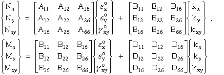
Substituting the [A], [B], and [D] matrices defined in equation (64) into equation (63)
results in the final relationship that defines the mechanical behavior of laminated
fiber-reinforced plate. Equation (63) shows the relationship between known in-plane
strains ( εox,
εoy,
γoxy ) and
curvatures ( kx,
ky,
kxy )
and unknown in-plane loads and moments.
And the inverse relates known in-plane loads to unknown in-plane strains and curvatures.
The [A], [B], and [D] matrices for the laminate are similar to the [Q] matrix for
the individual lamina. If you followed the basic ideas in this derivation it is
not difficult to understand how microscale lamina properties control the macroscale
laminate properties. In deed we now have a predictable way to control, and hence
design, the mechanical behavior of a laminate at the macroscale.
Like the lamina at the microscale, anisotropy of the laminate has a significant
effect on the mechanical behavior of the laminate. This can best be observed by
inspection of equations (65) and (66). If the individual lamina are stacked and
glued together such that the [B] matrix is zero then the mechanical behavior
exhibits a decoupling of moments and in-plane loads. For example curvatures only
affect moments and inplane strains only affect inplane load. On the other hand
it is not difficult to see that if [B] is not zero then there is coupling between
curvatures and inplane loads, and coupling also exists between inplane strains
and moments. This is rather peculiar. For example if we apply an inplane strain
to a specially configured laminate then the laminate can bend more then it
would extend ("stretch"). Similarly if we apply an inplane load the laminate will
twist. The later is actually used to an advantage by designers of aircraft
structures where aircraft wings, that are constructed by fiber-reinforced laminates,
are designed to twist into a predetermined aerodynamic angle-of-attack as
the wing bends and extends. This design methodology is called PASSIVE aero-elastic
tailoring. With "smart"-"intelligent" structures it is possible to insert
active piezoelectric layers into the laminate stacking sequence and ACTIVELY
control the mechanical behavior of the laminate. The degree of coupling is
controlled by the [A], [B], and [D] matrices.
In this section a few simple examples are presented that illustrate how simple
laminate configurations can provide predictable macroscopic mechanical behavior
by inspection of equations (65) and (66).
By inspection when [B] is zero, inplane loads and moments decouple in
equations (65) and (66).
Bi-directional laminates consist only of 0/90 degree lamina.
It is not difficult to show Q16 and Q26
For a large number of symmetric pairs, +θ
at +h and -θ at -h, D16 and D26
go to zero. Hence
Accept for a few simple cases outlined above, equations (65) and (66) are sufficiently
complex where the designer can not deduce a solution by observation. These equations
must be solved numerically, hence the designer must make educated guesses and
experiment by submitting multiple jobs and hopefully converge on a particular design.
To control the mechanical behavior of the laminate requires attention on controlling
the [A], [B], and [C] matrices. For complex stacking sequences this becomes difficult.
Many references on designing laminated structures exist. As an introduction we suggest
the reader look at Refs.[19,20]. To that end we provide an interactive tool below that
will allow the reader to experiment and design the desired laminate mechanical behavior.
In summary we have shown the significant role anisotropy has on the mechanical behavior
of laminates both at the microscale and macroscale. The bridge between the microscale
("lamina") and the macroscale ("laminate") is accomplished with analytic models of
laminated plate theory. In the theory of laminated plates we have ignored the stresses
and strains in the z-direction (thin-plate assumption). For thicker laminates at the
macroscale these stresses can not be ignored indeed these stresses are significant and
cause the formation of ply-cracks, see Figures 1,3, and 4. In the next section we
provide another model that predict stress singularities at the laminate free-edge.
Singularities at the laminated free-edge are also largely influenced by anisotropy
at the lamina microscale.
Mechanical behavior of thick laminated plates can be accurately predicted by simple
laminated plate theory, but the stresses within these thick laminates are not
accurately predicted by classical laminated plate theory. For thick laminates stress
singularities result in controlling the sequence of failure events that lead to the
ultimate fracture of the laminate. Figure 32 shows a typical sequence of damage events
that lead to ultimate fracture at the macroscale.
To accurately predict stress singularities in thick laminates we introduce the laminate
"Free-Edge" problem. In this section we provide:
Below is a description of the laminate geometry and finite element grid representation
used to define the stress "Free Edge" problem. The figure below shows the laminate stacking
sequence and FEM grid for a specific problem in Ref.[21].
NOTE: the enlarged area showing the smallest element of the F.E.Model at the free
edge is reaching the conceptual limit of the assumed homogeneous approximation ("continuum")
for material properties in each element at the free edge. The finite element mesh
superposed over a SEM photograph shows the heterogeneity of each graphite fiber
diameter, 5 microns, is observed as a fuzzy white region. Here we are pushing the limit
and assuming each element still behaves like a continuum with three fiber diameters
in the z-direction and ten fiber diameters in the horizontal y-direction. For FEM
elements smaller than this a continuum model can no longer be used. Instead a
different model needs to be created at Y/B > 0.998 where mechanical behavior is now
controlled by the individual fiber and matrix components. Hence the continuum
approximation breaks down at this point.
Example of results prior to First-Ply-Failure (FPF) in the WET ("water saturated") condition,
shown below, demonstrate the stress
singularity of the stress distribution of the normal stress in the z-direction along each
laminate interface. This singularity can only be accurately modeled up to Y/B=0.998 as a
continuum.
You might want to reproduce the results shown in this Figures 34 and 35 by going to the
interactive computer program. You will
also need to use the Laminated Plate Analysis
program which is used to convert the Nx=1900 lb./in. to a strain in the
x-direction. The strain in the x-direction, calculated by LELPA, is then used as the
out-of-plane strain normal to the H-Z plane in the form below. Notice that the
σz
stress reverses and becomes negative ("compressive") along the +45/-45 interface and
0/+45 interface most likely because of the combination of residual stresses caused by the
thermal contraction at low temperatures, ΔT=-180F, and swelling caused by moisture
absorption, ΔM=1.2% moisture.
All stresses at the laminate stress free edge and interior are summarized below in Table 4.
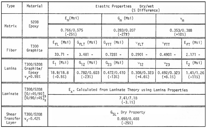
Elastic properties used to calculate these stresses are listed in Table 5.
In section 5.0 above a FEM model predicted stress free edge singularities in type-I
quasi-isotropic laminate, Ref.[21]. In section 6.0 below a FEM model
predicts stress singularities near a 90o ply crack terminating at the
0/90 interface in a type-II quasi-isotropic laminate, Ref.[1].
After the formation of a ply crack, see Figure 25, new singularities occur near the
ply crack tip. The growth of this crack can continue into the adjacent ply,
see Figures 1, 3, 4, and 5, or debond along the interface. Below we provide models that
demonstrate how anisotropy and residual stress can augment singularities near ply cracks
and influence how ply cracks grow and control laminate fracture strength.
In this section we provide:
Stress Analysis Summary: Details of the stress analysis is given in Reference [1].
Here we show a schematic of the laminate and finite element mesh that was used to model
a 90o ply crack in a [0/90/+45/-45]s laminate and the stress gradients
("concentrations") in the load bearing 0o ply near the ply crack tip, see also
Figures 3 and 4.
Summary: With the interactive computer program the reader can vary properties at the
microscale and observe the effect these changes have on the stress distributions near
the ply crack for two different types of quasi-isotropic laminates. Studying different
laminates would require creating different FEM meshes. Future examples will target
interactive FEM mesh generation. With this interactive computer program the reader
can reproduce these results and study how variations on elastic properties and other
properties at the microscale can influence the macroscopic stress state and influence
laminate fracture.
Similar to the stress "Free-Edge" FEM problem in section 5.0, the FEM model above
predicts stress singularities near the crack tip of a 90o ply crack in a
eight-layered type-II quasi-isotropic laminate. Below we introduce a FEM model with
a 90o ply crack in a [0/90]s laminate with and without a woven
macro-structure, Kriz Ref.[23]. These FEM models are complete where stresses plotted
in Ref.[23] are reproduced here, but graphical plots of these stress gradients are
not shown here because the interactive NPIB modules are under construction.
In previous sections we studied stresses near laminate stress free edges and ply cracks
that exist at an interface between two dissimilar anisotropic materials. These results
were predicted by a Finite Element Model (FEM) that did not include singularities.
Instead stresses gradients near the free edge and ply crack tips were approximated with
a high density FEM mesh near the singurality. In this section we introduce an analytic
model that predicts these singularites: 7.1) at a bimaterial interface intersecting a
stress free edge, see Figure 38, and, 7.2) at a ply crack tip intersecting an interface
seperating two dissimilar anisotropic media, see Figure 40. Both models are solved
using Stroh's method, Ref.[24]. These singularites can be introduced into enriched
FEMs that included a variety of different boundary conditions (BCs) without using high
density FEM meshes. With these enriched FEMs, stress intensity factors can be solved
for as unknowns along with the nodal displacements for each unique geometry and BCs.
Section 8 will outline how to create a finite element model with elements "enriched"
with these singularities, Benzley Ref.[29] and Heyliger & Kriz Ref.[30].
For both models, shown in Figs. 38 and 40, it is important to note that the singularity
coincides with the origin of the coordinates. Hence each model has a unique coordinate
system. Since the objective here is to reproduce published results of these two models
the same coordinate system established by Ting et al. will be used. This choice will
require rederivation of an arbitray rotation in the 1-2 plane for orthorhombic
symmetry outlined in section 4.1. The derivations below will follow the notation and
procedures outlined by Ting et al, Refs. [25] and [26]. The notes below will expand on
the solution introduced by Ting et al. by developing the numerical approach to solve
for these singularities. These singularities were also calculated by using Green's
functions at dissimilar anisotropic material interfaces terminating at a stress free
edge, Tewary & Kriz Refs. [27] and [28].
T.C.T. Ting and S.C. Chou, Ref.[25], used Stroh's method to solve for the singularity
where the interface seperates two dissimilar anisotropic regions and terminates at a
stress free edge, see Figure 38. Here we only expand on the development of the
numerical solution and use the same notation in Ref.[25] except the exponent on the
radius, r, is changed from, δ, to -k similar to the exponent in Ref.[26].
The solution is organized into three parts:
1) transformation of the fourth order
stiffness tensor, Cijkl, for arbitrary rotation in the 1-3 plane,
see eqn 35 Ref.[25],
2) calcuate eigenvalues, pk, and
eigen vectors, νi and τij, from equations (9) and
(10) Ref.[25], and
3) calcuate exponent (singularity)
on radius, r, from the determinate of equations that are created when equations
(30) and (31) of Ref.[25] are combined with appropriate boundary conditions.
Below we expanded and simplify eqn. (10) into an eigenvalue problem that we
can solve by using IMSL scientific subroutines. Combining equations (11) and (12)
from Ref.[25] along with the rotated transformed stiffnesses, yields
Substituting eqn (68) into eqn (10) of Ref.[25] yields
Note that PL exists in every term of the coefficient matrix
in eqn. (69) who's determinate yields a cubic characteristic equation in
PL2. Although it is possible solve for the roots of
this characteristic equation, numerical solutions to this type of problem
yield more accurate eigenvalues. Hence eqn.(69) is further developed into
an eigenvalue problem where PL are complex eigenvalues and
their corresponding complex eigenvectors, ν
i,L, where the ,L subscript associates the eigenvector with the
appropriate eigenvalue (L=1,2,3). The L is not a free indice and the comma
does not imply differentiation
The eigenvalue format is
It is possible to expand equation (69) into the form of equation (70).
First we rewrite equation (69).
where we can write equation (71) in abbreviated notation.
Multiply equation (72) by the inverse of the coefficient matrix, [A'],
yeilds.
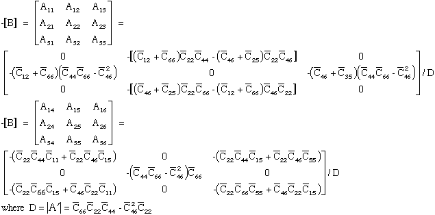
where [A']-1[A'] becomes the indentity matrix [I], and matrices
[B'] and [C'] are premultiplied by [A']-1 and become [B] and [C]
respectively.
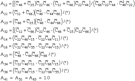
The array [A] in eqn.(70) can be constructed such that
where the nonzero components in array [A] of eqn.(70) are summarized below.
To show eqn.(70) and eqn.(73) are equivalent requires the following expansion.
First substitute eqn.(75) into eqn.(70) where the {Z} eigenvectors are partioned
into Xi and Yi components.
where
Equation (77) can be rewritten interms of Xi and Yi
components.
Expanding eqn.(79) yields two equations
These two equations can be combined into one equation by substituting
for Xi, hence eliminating Xi, and rearranging terms.
where comparing equations (81) and (73) yield the necessary eigenvalues and
eigenvectors
Comparing equations (81) and (73) verifies that equation (70) can be
used to solve for PL as eigenvalues instead of roots to the
characteristic equation derived from the determinate of the coefficient
matrix in equation (69). Both eigenvalues, PL, and eigenvectors
from equation (81) will be used in the next section to calculate the
singular exponent. IMSL routines EVCRG are used to solve equation (70) and
EPIRG is used to obtain a performance index for the solutions.
Using Stroh's method Ting et al., Ref.[25], obtained the functional form for
displacements and stresses.
where again we note that ,L does not imply differentiation and L is not a
free indice but is used as a subscript to identify eigenvectors associated
with the L-th eigenvalue. Here L is assigned 1,2,3 corresponding to the three
eigenvalues of eqn.(69).
The equations above have been slightly modified. The exponent has been changed
from δ to -k and the
coefficients, ML and NL have been renamed aL
and a'L.
To solve for the exponent singularity, k, we create
a systems of 12 linear equations from Ting's equations (30) and (31) and the
boundary conditions listed below. Coefficients of these equations are written in
terms of k and solved for k
as a root to the determinate of the coefficient matrix of these equations. Since
the solution is to find only one of the roots between 0.0 and 1.0, this root is
first approximated by calculating the determinate as a function
("function-subroutine") of k where a value for
k is incremented from 0.0 to 1.0 until the determinate
changes sign (+/-). Within this interval a root exists. With an approximation
for the root interval other IMSL routines can be used to obtain a more accurate
solution for k. Next we construct the twelve equations
for the boundary conditions defined in Fig. 38.
The boundary conditions are:
From these boundary conditions 12 equations are generated whose coefficients are
functions of elastic properties and the exponent on the radius vector whose
origin is located at the crack tip where the singularity exists. Below we
generate this coefficient matrix.
Boundary condition 1:
Boundary condition 2:
Boundary condition 3:
Boundary condition 4:
The blocks defined above are substituted into the schematic shown below.
IMSL routine ZBREN is used to find a solution (root) to the determinate
of the coefficient matrix shown in Fig. 39. The ZBREN requires an initial
guess where the determinate changes sign in the interval from 0 to 1.0.
Hence a function subroutine, F, is setup which calculates the determinate
using IMSL routines LFTRG and LFDRG.
With the interactive computer program provided above the student can reproduce the
singularities tabulated below. In particular the default values set in the NPIB
form of the computer program is configured to calculate the singularity of
2.9388 x 10⁻² for
θ'=0 and θ=75 with the
Pipes-Pagano approximation for elastic properties:
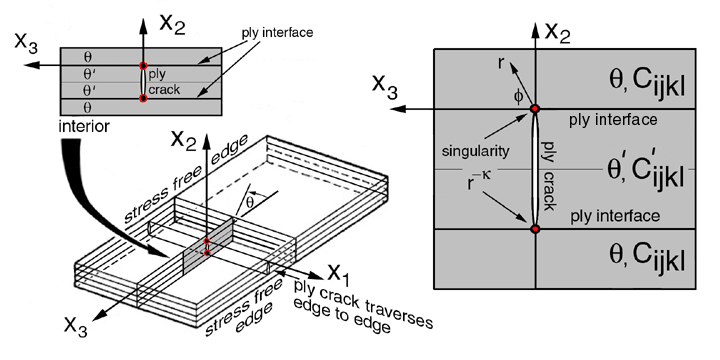
T.C.T. Ting and Hoang, Ref.[26], used Stroh's method to solve for the singularity
at a ply crack tip acting normal to an interface seperating two dissimilar anisotropic
regions, see Figure 40.
It is important to note that singularities coincide with the coordinate system origin.
Hence each interface singularity has a unique coordinate system. Since the objective
here is to reproduce published results the same coordinate system established by Ting
et al. will be used. This choice will require rederivation of an arbitray rotation
in the 1-2 plane for orthorhombic symmetry outlined in section 4.1. The derivations
below will follow the notation and procedures outlined by Ting et al, Ref.[26]. For
this module we have expanded on the solution introduced by Ting et al. and developed
the numerical approach to solve for these singularities.
The solution is organized into three parts:
1) transformation of fourth
order stiffness tensor, Cijkl, for arbitrary rotation in the 1-3 plane,
see eqn 35 Ref.[25],
2) calcuate eigenvalues,
pk, and eigen vectors, νi and τij,
from equations (9) and (10) Ref.[25], and
3) calcuate exponent, k (singularity) on radius, r, from
determinate of equations that are created when equations (21) and (22) of Ref.[26]
are combined with the appropriate boundary conditions equation (36) of Ref.[26].
NOTE: The geometry shown in Fig.40 results in a set of boundary
conditions different then those used in the previous section 7.1.
From these boundary conditions 18 equations are generated. Coefficients are functions
of elastic properties and the exponent on the radius vector whose origin is located at
the crack tip where the singularity exists. Unlike boundary conditions for the free
edge problem of section 7.1, there is an additional notation where + or - appear as
superscripts on variables that indicates these variables exist in regions
x3 > 0 and x3 < 0 respectively.
Partial results from Ting et al. Ref.[26] are listed below in Table 7 with the
Pipes-Pagano approximation for elastic properties:
We provide an interactive computer program module below where you can reproduce
these results. The default values in the NPIB form will generate results highlighted
in red in the Table above for θ=30 and θ'=60 which uses the Pipes-Pagano
approximation for elastic properties. Unfortunately there are unresolved errors in
the Fortran computer program (plysing.f) in module15b that predicts singularities
listed in Table 7 above.
Singularites predicted for the stress "Free Edge" problem in section 7.1 have been
reproduced, listed in Table 6, and can be used in enriched finite elements in
Section 8.0 below.
Outline how enriched finite elements are used to augment existing nonsingular
finite elements with singularities that exist at crack tips, Benzley Ref.[29].
Use this enriched FEM to model crack tip singularities in a homogeneous
isotropic material and compare numerical results with analytic results that
predict Stress Intensity factors for Mode-I and Mode-II, Heyliger & Kriz Ref.[30].
Predict stress gradient near holes in an anisotropic and isotropic
plate and compare results with Mizra & Olson Ref.[31].
Introduction to 1-D isotropic wave propagation: Analytic and Numerical Models
Introduction to 2-D anisotropic wave propagation: Numerical models
4.2 Introduction to Mechanical Behavior of Laminates (Laminate Plate
Theory): Analytic Model
With laminated plate theory we bridge the scale of modeling mechanical
behavior from the micro "lamina" scale to the macro "laminate" scale. Figure
25 shows the construction of a laminated plate with individual lamina layers.
In practice laminated plates consist of hundreds stacked lamina but here we
study simple laminated structures.

Figure 25. Lamina-Laminate Definitions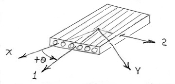
Figure 26. Lamina axes defined

(44)

(45)

(46)

(47)

(48)

(49)

(50)

(51)

(52)

(53)

(54)
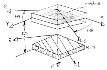
Figure 27. Lamina-Laminate Configuration Geometry Defined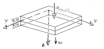
Figure 28. Thin Plate Deflections

(55)

(56)

(57)
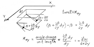
Figure 29. Exaggerated Thin Plate Deflections and Twists Defined

(58)

(59)

(60)
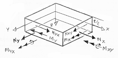
Figure 30. Laminate Plate In-Plane Loads and Moments Defined

(61)

(62)
(63)

(64)
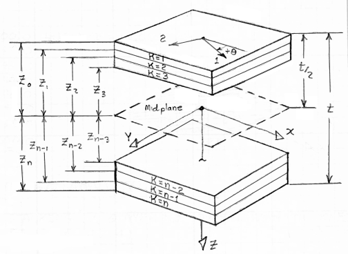
Figure 31. Lamina Positions Defined in the Laminate for Integration of Resultant Loads

(65)

(66)
Inplane loads {N} only produce inplane strains {ε}
and inplane moments {M} only produce
curvature {k}
are zero. Hence A16 and A26 are also zero and consequently
the inplane shear strain {γ} decouples
from the inplane normal strains. Therefore shearing loads can only produce
shearing strains and
inplane normal loads can only produce inplane strains
moments {Mx} & {My} and torque {Mxy} decouple
so that bending caused by moments do not
introduce twisting and torque that causes twisting does not introduce bending.
5.0 Laminate Singularities Caused by Anisotropy: "Free-Edge Problem": FEM Model
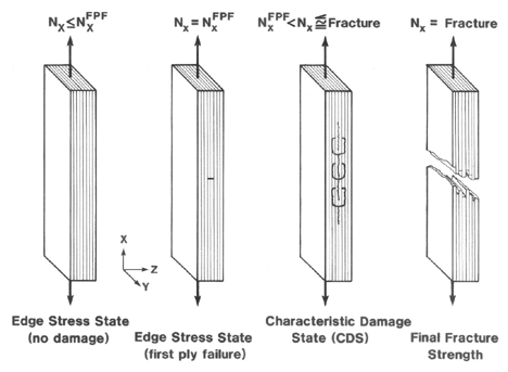
Figure 32. Typical sequence of damage events leading to laminate fracture
, Ref.[22].
results are compared with Pipes and Pagano Finite Difference Model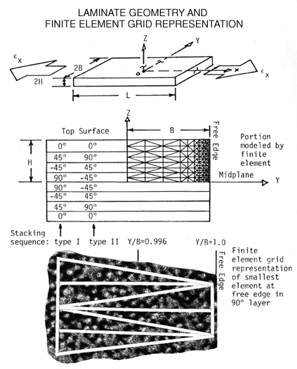
Figure 33. Laminate geometry and FEM grid defined for "Free-Edge" problem, Ref.[21].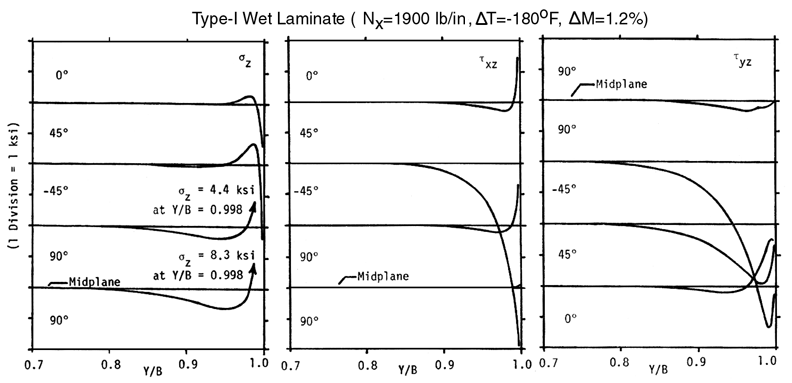
Figure 34. Sample results of laminate edge-stress singularities, Ref.[21].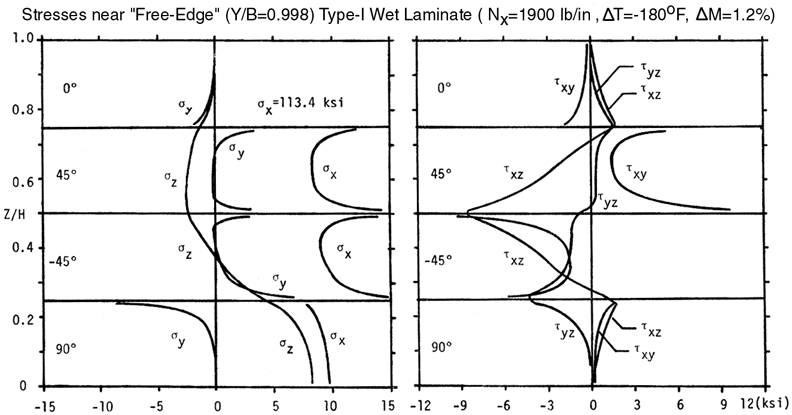
Figure 35. Sample results of stresses at laminate stress free edge, Ref.[21].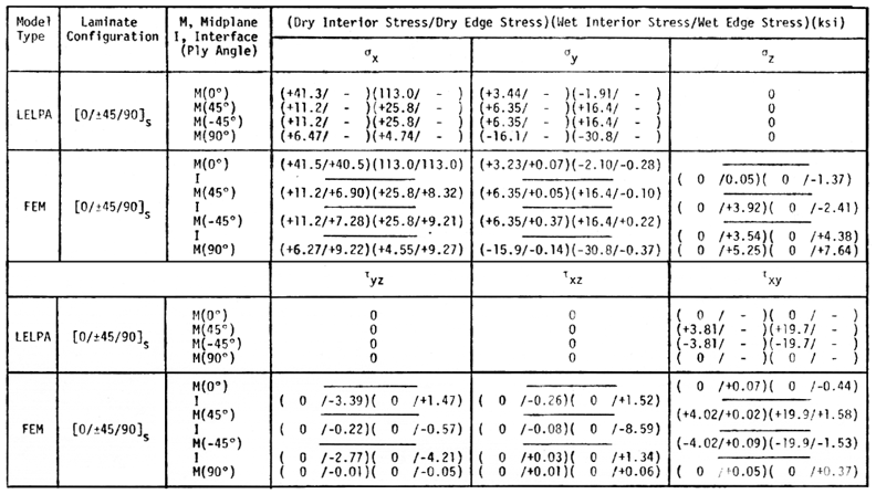
6.0 Laminate Singularities Caused by Ply Cracks: FEM Model
Compares stress analysis (FEM program) with fractographs and statistical
analysis of fracture strengths.
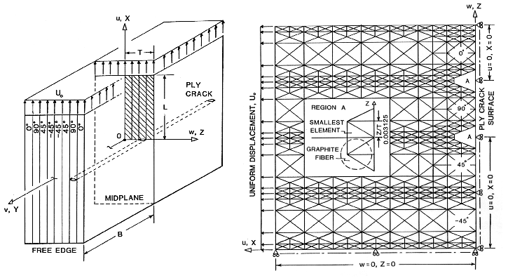
Figure 36. Schematic and FEM Grid of Ply Crack in a [0/90/+45/-45]s laminate, Ref.[1]
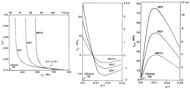
Figure 37. Mode I stresses in the 0 degree load bearing ply above the ply crack, Ref.[1]
7.0 Cracks Near Interfaces Between Dissimilar Anisotropic Materials
7.1 Stress free edge singularities:
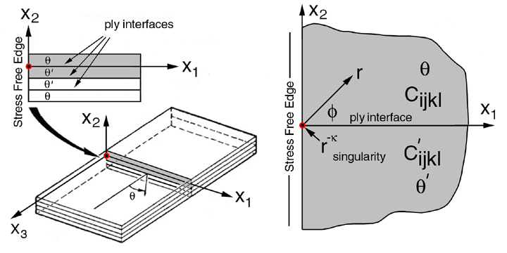
Equations summarized above are compiled into a Fortran computer program (edgesing.f)
which is provided below as an interactive module (Module15a). This same program can
be accessed and downloaded from Module15a listed in the
Microstructure Interactive Computer Program Modules
Table section of the CRCD pages.
7.1.1 Tensor Transformation Cijkl in 1-3 plane:
Hand-written notes are provided for the
transformation of the fourth order stiffness tensor for arbitray rotations
in the 1-3 plane.
7.1.2 Calculate Eigenvalue/Eigenvectors, pk /
νi and τij:
We start with equations (9) and (10) in Ref.[25].

(9) Ting

(10) Ting

(11) Ting

(12) Ting

(67)
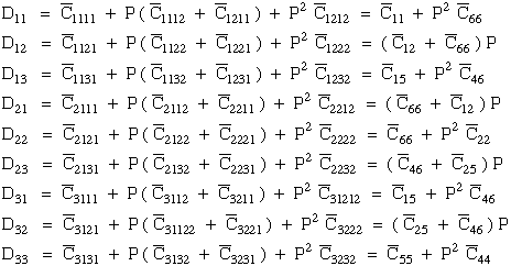
(68)

(69)

(70)

(71)

(72)

(73)
(74)

(75)
(76)

(77)

(78)

(79)

(80)

(81)

(82)
7.1.3 Calculate Singular Exponent, -k:

(30) Ting

(31) Ting

(26) Ting

(83)


(84)


(85)


(86)


(87)
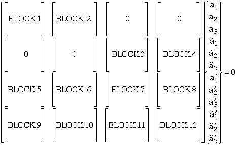
Figure 39. Block schematic of system of equations for determining singularity
where bimaterial interface terminates at a stress free laminate edge.
G12=G13=G23=+0.850E+06
ν21=
ν31=
ν32=+0.210E+00
Exponent
of r-kθ'=0
θ'=90
θ'=-θ
θ=0
-
3.3388 x 10⁻²
-
θ=15
1.3528 x 10⁻⁴
3.2814 x 10⁻²
6.4322 x 10⁻⁴
θ=30
2.6286 x 10⁻³
2.8682 x 10⁻²
1.1658 x 10⁻²
θ=45
9.6461 x 10⁻³
2.0575 x 10⁻²
2.5575 x 10⁻²
θ=60
1.9866 x 10⁻²
1.0519 x 10⁻²
2.3346 x 10⁻²
θ=75
2.9388 x 10⁻²
2.6785 x 10⁻³
8.9444 x 10⁻³
θ=90
3.3388 x 10⁻²
-
-
7.2 Ply Crack singularities:
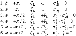
(88)
G12=G13=G23=+0.850E+06
ν21=
ν31=
ν32=+0.210E+00
Exponent
of r-kθ=0
θ=15
θ=30
θ=45
θ=60
θ=75
θ=90
θ'=90
.676635
.500212
.5.676012
.502156
.500222.672441
.505068
.500236.660488
.504813
.500227.630471
.502297
.500314.567537
.500314
.500048.5
θ'=75
.675051
.500189
.433918.665411
.500305
.446234.646234
.500401
.466560.616354
.500401
.485037.571159
.500269
.496300.5
.499859
.499688
.4322561
θ'=60
.665263
.499839
.379767.642118
.500352
.404849
.605628
.500735
.441810.557636
.500673
.477316.5
.503704
.499085
.430024.498608
.497668
.371402
θ'=45
.643963
.499012
.369508.606474
.500092
.407075.556388
.500639
.456342.5
.522801
.498293
.443947.515052
.496531
.388842.495691
.495008
.345965
θ'=30
.609394
.498562
.391694.557954
.499986
.442491.5
.543655
.498192
.445399.558434
.495380
.400299.533668
.493226
.364378.494600
.492252
.339747
θ'=15
.560499
.499279
.438704.5
.557552
.498554
.444039.592813
.495627
.400073.595139
.492603
.369244.553905
.490548
.349787.497659
.489828
.340358
θ'=0
.5
.562178
.498904
.441309.609785
.496201
.397243.631434
.493110
.367864.620457
.490626
.350305.566078
.489298
.342401.5
.489038
.341108
8.0 Cracks in Homogeneous Isotropic Materials
9.0 Stress Concentrations in Homogeneous Anisotropic Plates
10.0 Wave Propagation in Homogeneous Isotropic/Anisotropic Materials
11.0 References
Send comments to: rkriz@vt.edu
Ronald D. Kriz, Short Bio
Engineering Science and Mechanics
College of Engineering
Virginia Tech
Blacksburg, Virginia 24061
Web Content Chronology:
Created ESM Dept On-Campus Web-server November 1997 / Modified December 2000
http://www.jwave.vt.edu/~rkriz/crcd/lectures/OnePageLect.html
Moved to Off-Campus Web-server November 2014
http://www.jwave.rkriz.net/crcd/kriz/lectures/OnePageLect.html
DVD: ESM Content Archive:
DVD-ESM-Archive/esm/ESM-DVD/classes/ESM5344/ESM5344_NoteBook/crcd/lectures/OnePageLect.html